Example scripts
This is an index of the example scripts in the examples directory in the repository. The links point to the file preview on github.
Short index
a acic b bart barteasy c d dft doubleint e even f fourier g h i j k l m n o pdf1 pdf10 pdf2 pdf3 pdf4 pdf5 pdf6 pdf7 pdf8 pdf9 q r s t u v w x y z
Index with figures
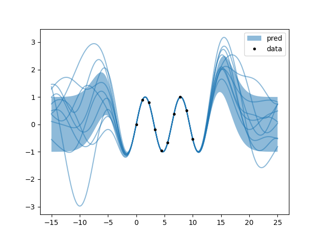
a.py: EXAMPLE A.
Where the oscillating nature of an unknown function is revealed from but a few points, though only to a certain distance.
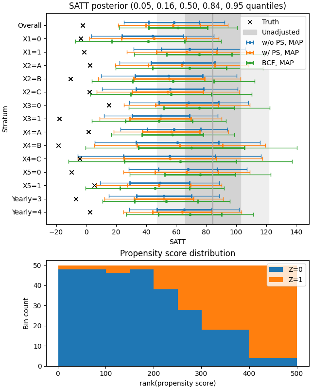
acic.py: Analyze a dataset from the ACIC 2022 Data Challenge using the BART kernel.
Website: https://acic2022.mathematica.org
Article: Dan R.C. Thal and Mariel M. Finucane, “Causal Methods Madness: Lessons Learned from the 2022 ACIC Competition to Estimate Health Policy Impacts,” Observational Studies, Volume 9, Issue 3, 2023, pp. 3-27, https://doi.org/10.1353/obs.2023.0023
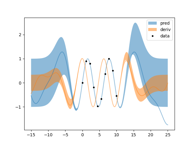
b.py: EXAMPLE B.
Where it is discovered that the derivative of the unknown function is orthogonal to the function itself, and furthermore that it is orange instead of blue.
bart.py: Example usage of the BART kernel to replace the standard BART MCMC algorithm.
barteasy.py: BART with the simplified subpackage.
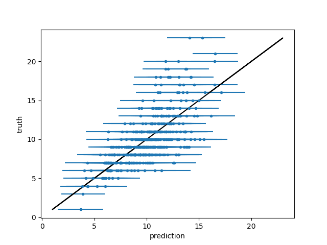
c.py: EXAMPLE C.
Where a nonlinear transformation hides the true height of some crosses.
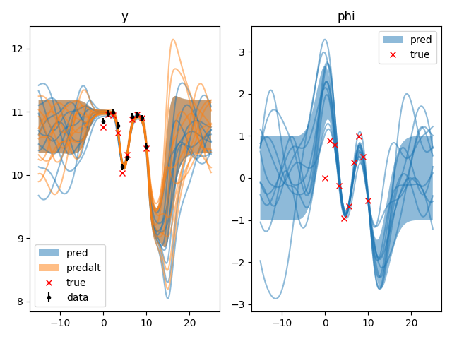
d.py: EXAMPLE D.
Where the primitive of our function takes some freedom to move up and down.
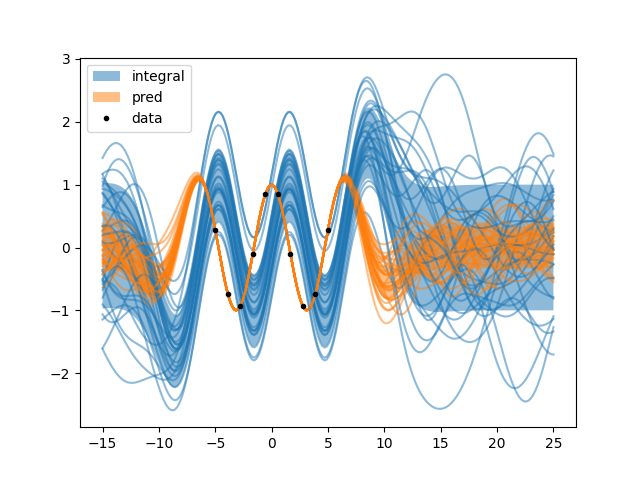
dft.py: Constrain the discrete Fourier transform of a periodic process. Shows how to use GP.addlintransf.
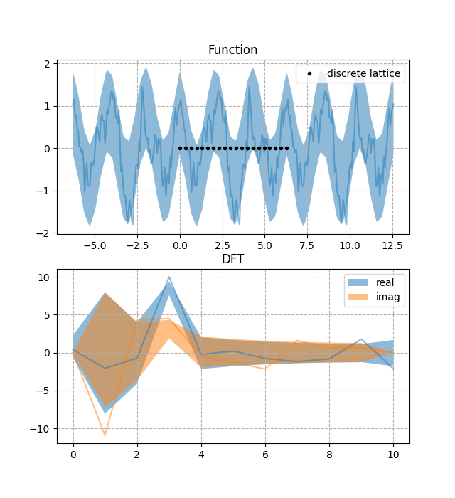
doubleint.py: Test of double integral constraint
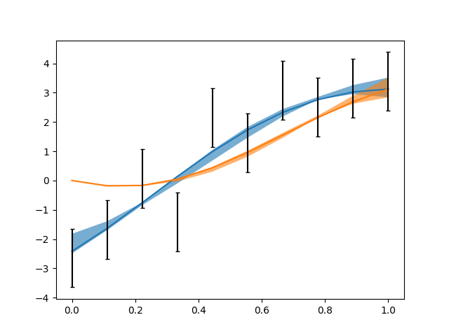
e.py: EXAMPLE E.
Where observing both a function and its derivative put some restraint on their behaviour.
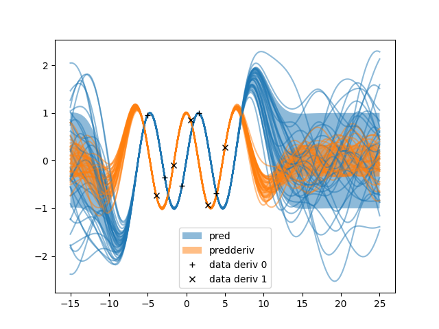
even.py: Split a function into even and odd parts.
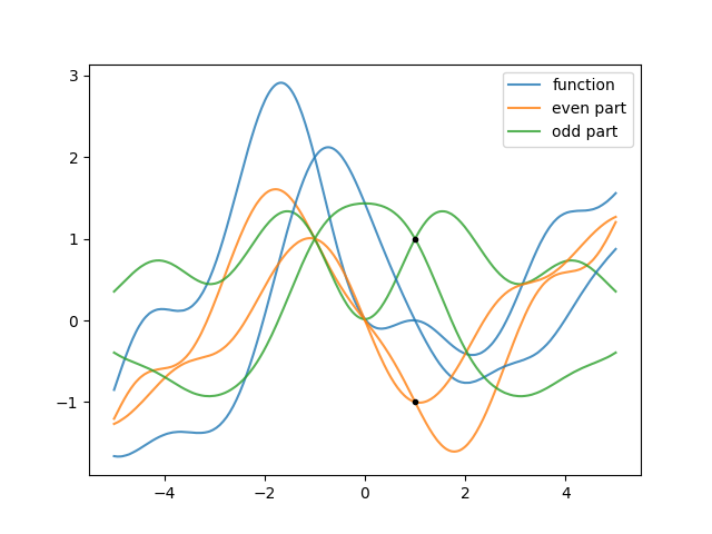
f.py: EXAMPLE F.
Where apparently in these times it is not anymore possible to know exactly where one gentleman’s function will pass.
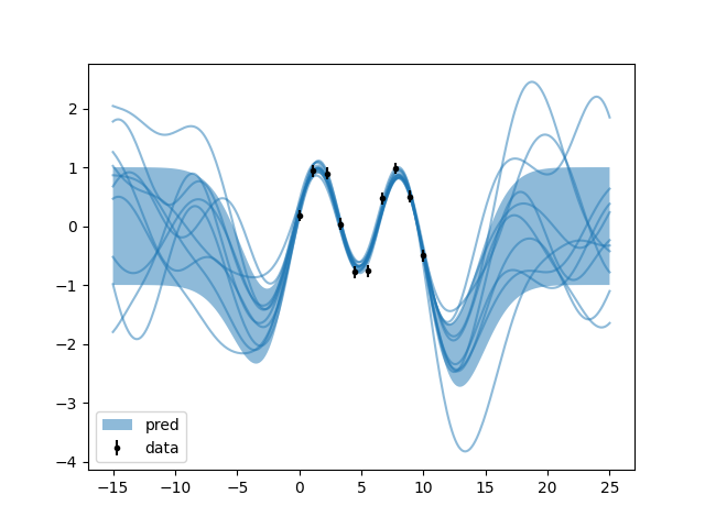
fourier.py: Constrain the values of Fourier series coefficients
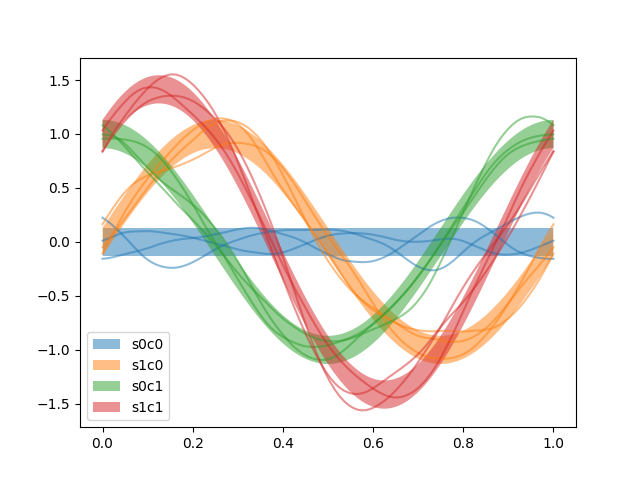
g.py: EXAMPLE G.
Where two ways of expressing one’s beliefs are compared and found, satisfactorily, to be quite similar.
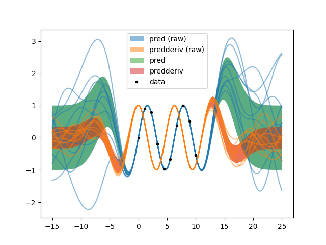
h.py: EXAMPLE H.
Where at first sight nothing has changed, but behind the scenes important information has been lost forever.
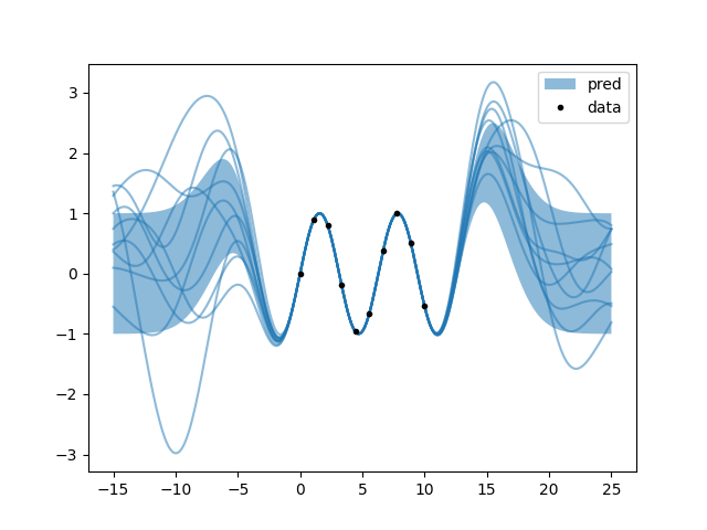
i.py: EXAMPLE I.
Where, due to obscure political reasons, we insist on forgetting important details that a reasonable man’s mind would be fond of recalling later.

j.py: EXAMPLE J.
Where the excessive smoothness of the prediction is found not to satisfy our manly tastes.
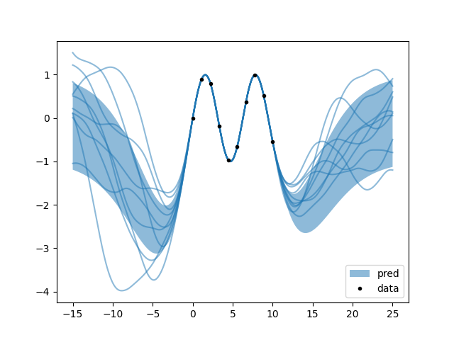
k.py: EXAMPLE K.
Where lady K finds out that every gentleman hides his rougher corners in his derivative.
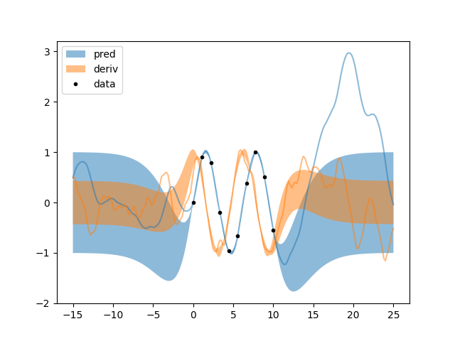
l.py: EXAMPLE L.
Where two formulas give the same results and so math triumphs once again.
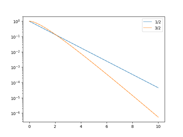
m.py: EXAMPLE M.
Where we discover that, unlike elephants, Matérn processes prefer to forget after less than one data step.
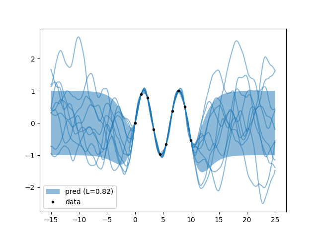
n.py: EXAMPLE N.
Where we wonder how much a derivative is allowed to do her own business compared to her mistress.
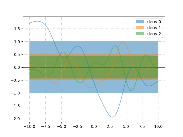
o.py: EXAMPLE O.
Where mister N’s enquiry is repeated by different means.
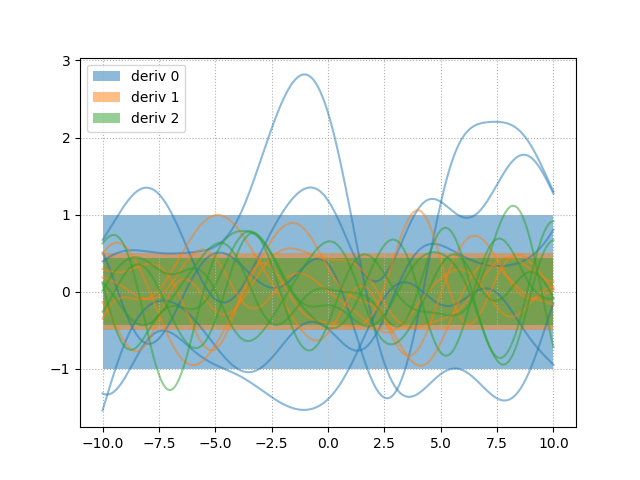
pdf1.py: Fit of parton distributions functions (PDFs)
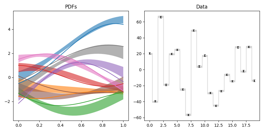
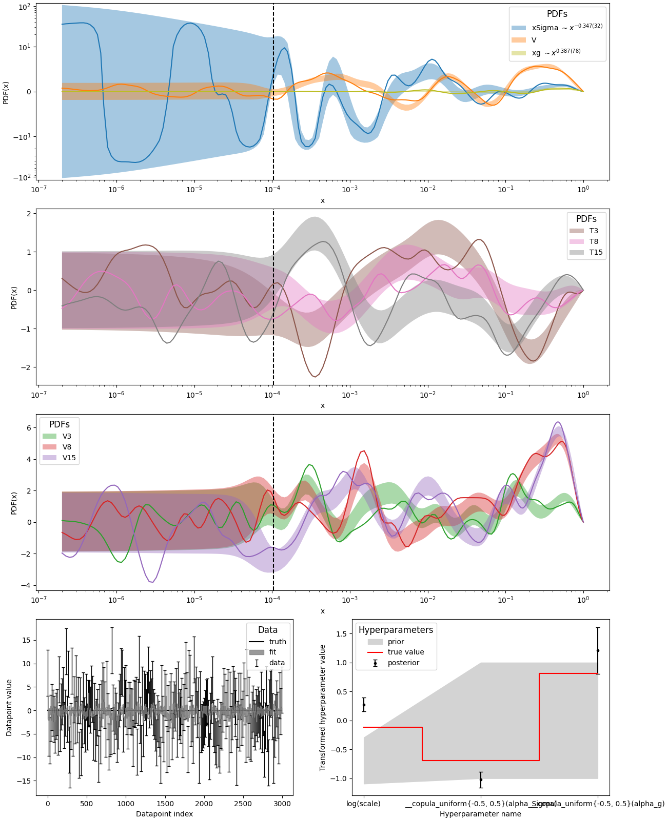
pdf10.py: Fit of parton distributions functions (PDFs)
Like pdf9, but with per-function hyperparameters
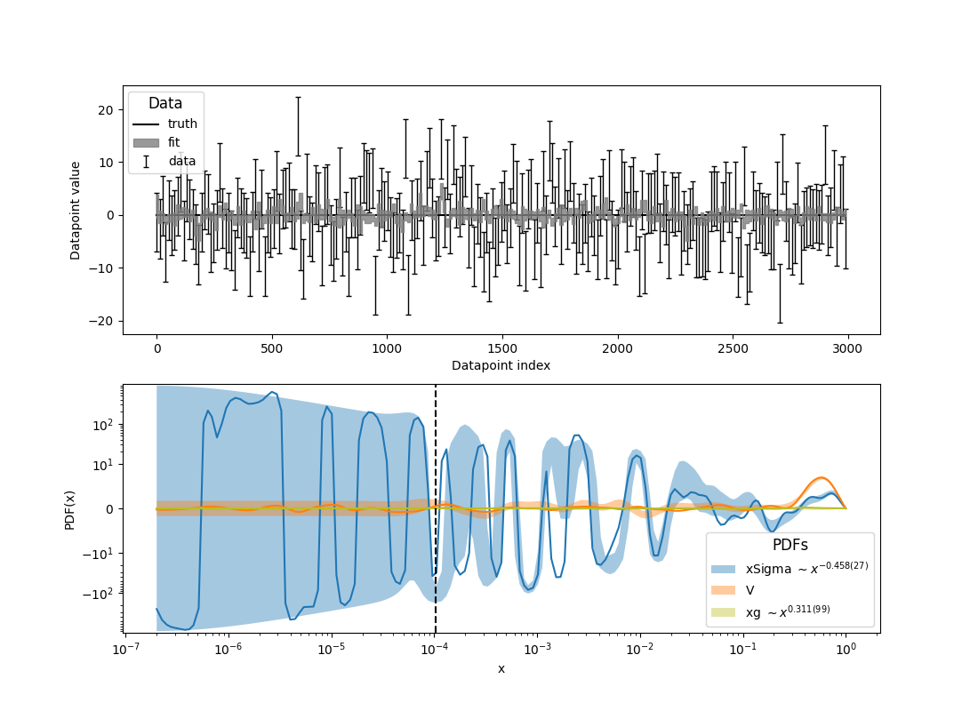
pdf2.py: Fit of parton distributions functions (PDFs)
The difference from pdf1.py is that we define the transformation on processes instead of on their finite realizations
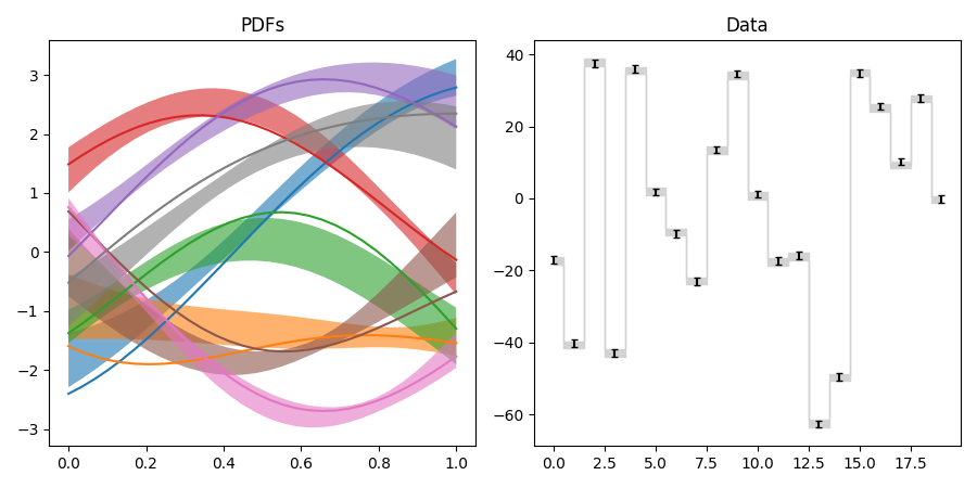
pdf3.py: Fit of parton distributions functions (PDFs)
Like pdf2, but with correct integral constraints and naming this time
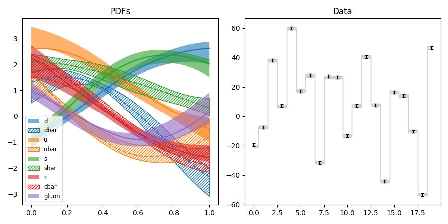
pdf4.py: Fit of parton distribution functions (PDFs)
Like pdf3, but with hyperparameters
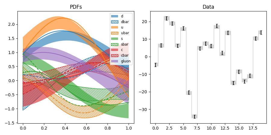
pdf5.py: Fit of parton distributions functions (PDFs)
Like pdf3, but with nonlinear data
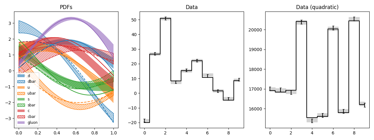
pdf6.py: Fit of parton distributions functions (PDFs)
Like pdf5, but with uncertainties on M and M2
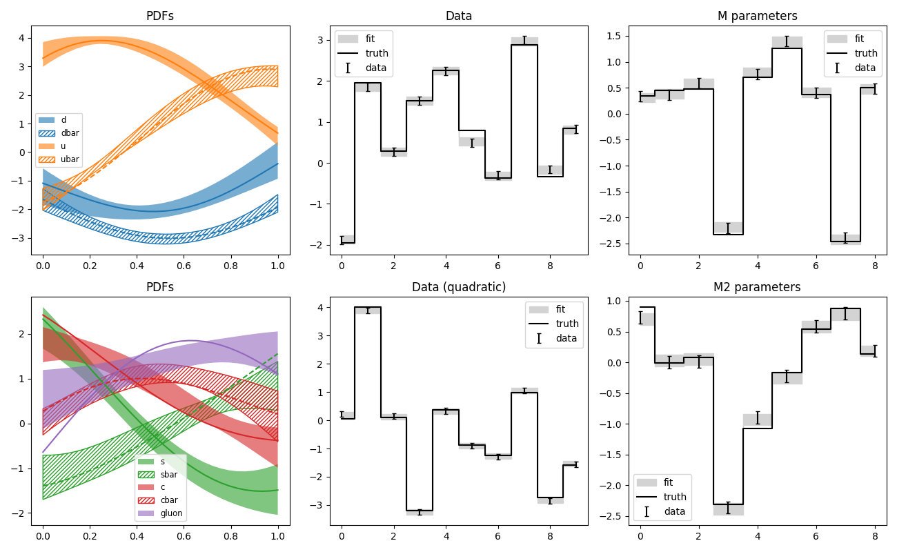
pdf7.py: Fit of parton distributions functions (PDFs)
Like pdf6, but with hyperparameters
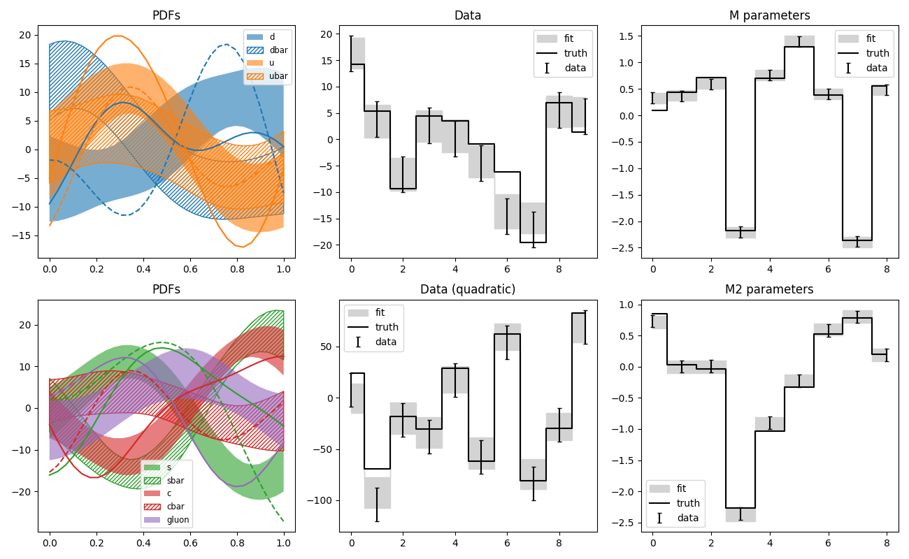
pdf8.py: Fit of parton distributions functions (PDFs)
Like pdf7, but with more realistic PDFs
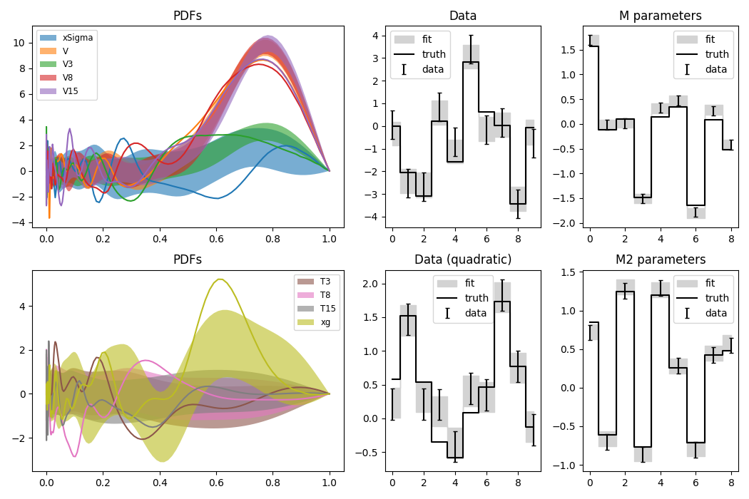
pdf9.py: Fit of parton distributions functions (PDFs)
Like pdf8, but only with linear data
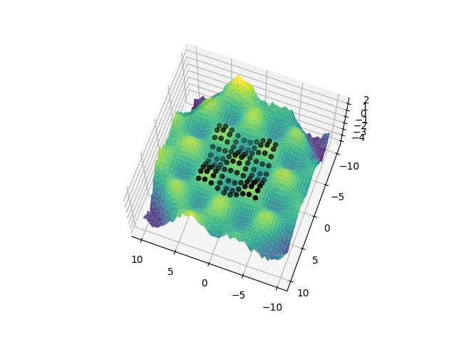
q.py: EXAMPLE Q.
Where we extend a pattern of waves in space, but do not dare look too far from our data.
r.py: EXAMPLE R.
Where we decide to introduce a strong anisotropy despite evidence of its absence.
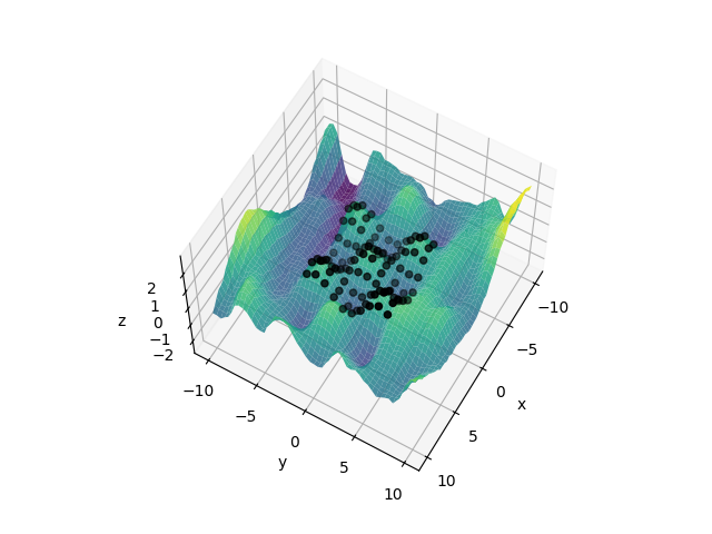
s.py: EXAMPLE S.
Where different coordinates unite together under a single field name.
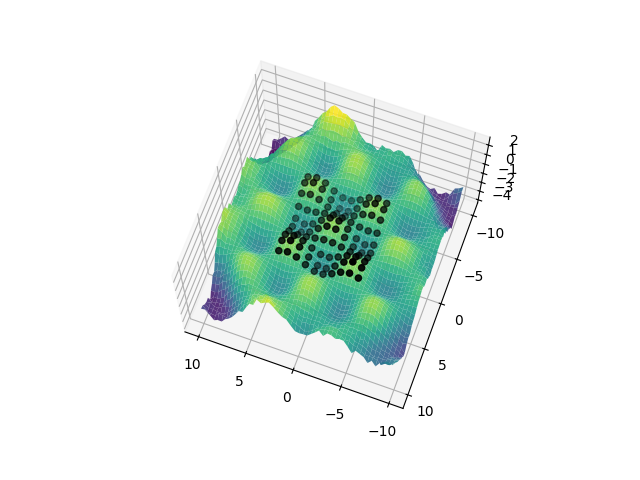
t.py: EXAMPLE T.
Where we pretend to discover that two series of events were in fact one the delayed and imperfect copy of the other.
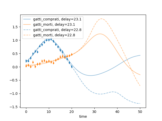
u.py: EXAMPLE U.
Where we infer the temporal scale of a process assuming another process is correlated with its derivative.
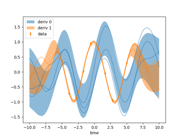
v.py: EXAMPLE V.
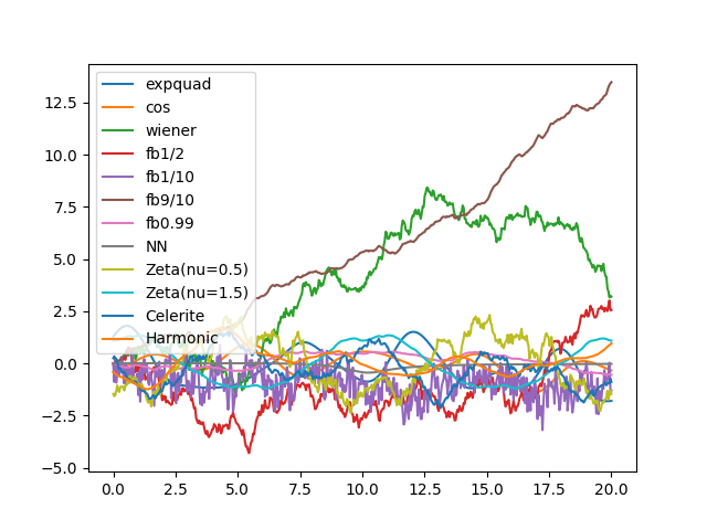
Where we go on an expedition to survey the many and wondrous kernels that inhabit our software.
w.py: EXAMPLE W.
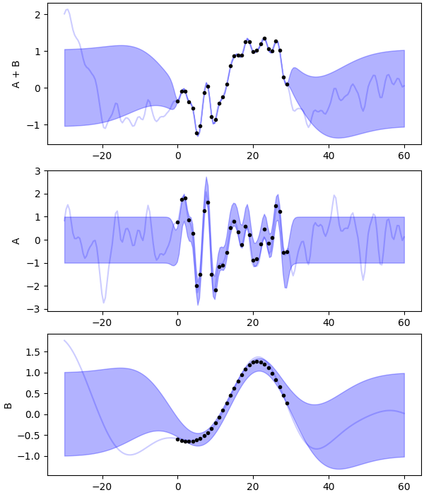
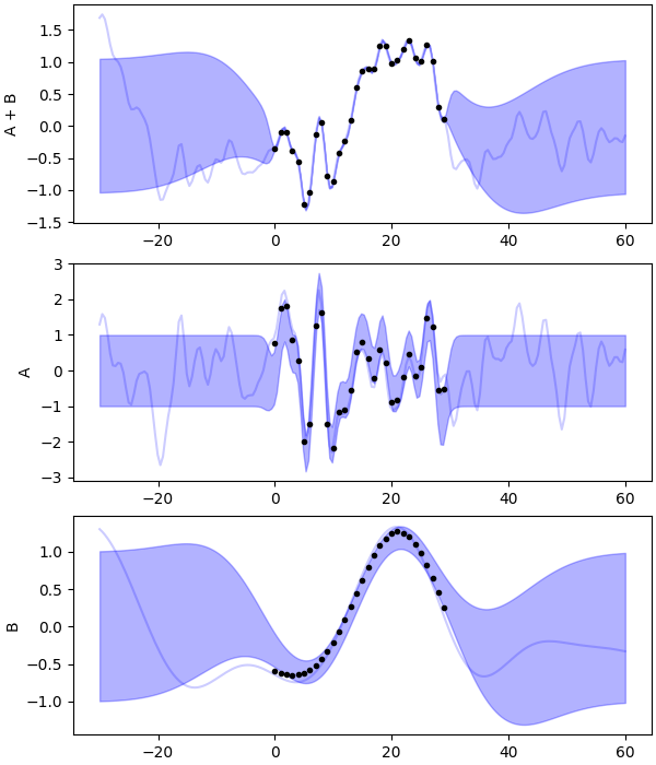
Manually split a process as a sum of two processes, using an additional index in the input space.
x.py: EXAMPLE X.
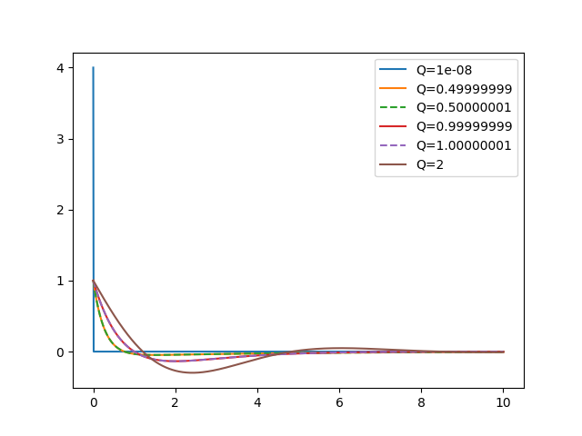
Where the derivatives of an interesting correlation function are put to harsh a trial.
y.py: EXAMPLE Y.
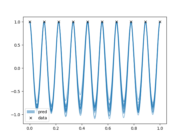
Where a Zeta kernel forces some random samples to have zero mean.
z.py: EXAMPLE Z.
Where we sail in an infinite dimensional space to sum two numbers.
