Predefined kernels
This is a list of all the specific kernels implemented in lsqfitgp.
Kernels are reported with a simplified signature where the positional arguments
are r or r2 if the kernel is isotropic, delta if it is stationary, or x,
y for generic kernels, and with only the keyword arguments specific to the
kernel. All kernels also understand the general keyword arguments of
CrossKernel (or their specific superclass), while there are no positional
arguments when instantiating the kernel and the call signature of instances is
always x, y.
Example: the kernel GammaExp is listed as GammaExp(r, gamma=1). This means
you could use it this way:
import lsqfitgp as lgp
import numpy as np
kernel = lgp.GammaExp(loc=0.3, scale=2, gamma=1.4)
x = np.random.randn(100)
covmat = kernel(x[:, None], x[None, :])
On multidimensional input, isotropic kernels will compute the euclidean distance.
For all isotropic and stationary (i.e., depending only on \(x - y\)) kernels
\(k(x, x) = 1\), and the typical lengthscale is approximately 1 for default
values of the keyword parameters, apart from some specific cases like
Constant.
Warning
You may encounter problems with second derivatives for CausalExpQuad,
FracBrownian, NNKernel, and with first derivatives too for Wendland
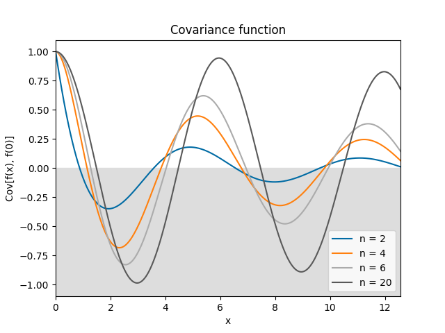
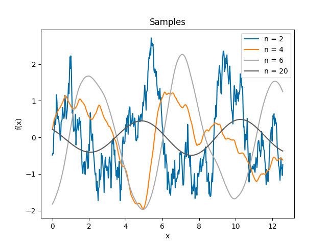
(but only in more than one dimension). Color stops working for
\(n > 20\).
Index
Isotropic kernels
Stationary kernels
Other kernels
Documentation
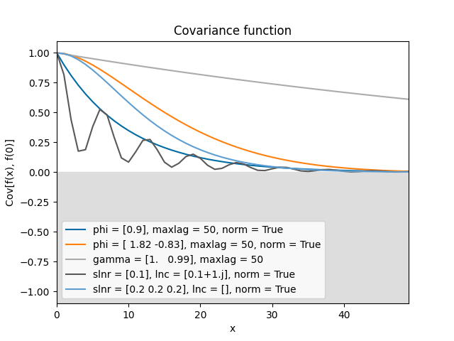
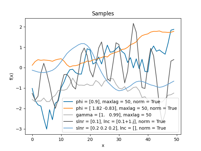
- class lsqfitgp.AR(**kw)[source]
Discrete autoregressive kernel.
You have to specify one and only one of the sets of parameters
phi+maxlag,gamma+maxlag,slnr+lnc.- Parameters:
- phi(p,) real
The autoregressive coefficients at lag 1…p.
- gamma(p + 1,) real
The autocovariance at lag 0…p.
- maxlagint
The maximum lag that the kernel will be evaluated on. If the actual inputs produce higher lags, the missing values are filled with
nan.- slnr(nr,) real
The real roots of the characteristic polynomial, expressed in the following way:
sign(slnr)is the sign of the root, andabs(slnr)is the natural logarithm of the absolute value.- lnc(nc,) complex
The natural logarithm of the complex roots of the characteristic polynomial (\(\log z = \log|z| + i\arg z\)), where each root also stands for its paired conjugate.
In
slnrandlnc, the multiplicity of a root is expressed by repeating the root in the array (not necessarily next to each other). Only exact repetition counts; very close yet distinct roots are treated as separate and lead to numerical instability, in particular complex roots very close to the real line. An exactly real complex root behaves like a pair of identical real roots. Two complex roots also count as equal if conjugate, and the argument is standardized to \([0, 2\pi)\).- normbool, default False
If True, normalize the autocovariance to be 1 at lag 0. If False, normalize such that the variance of the generating noise is 1, or use the user-provided normalization if
gammais specified.
Notes
This is the covariance function of a stationary autoregressive process, which is defined recursively as
\[y_i = \sum_{k=1}^p \phi_k y_{i-k} + \epsilon_i,\]where \(\epsilon_i\) is white noise, i.e., \(\operatorname{Cov}[\epsilon_i, \epsilon_j] = \delta_{ij}\). The length \(p\) of the vector of coefficients \(\boldsymbol\phi\) is the “order” of the process.
The covariance function can be expressed in two ways. First as the same recursion defining the process:
\[\gamma_m = \sum_{k=1}^p \phi_k \gamma_{m-k} + \delta_{m0},\]where \(\gamma_m \equiv \operatorname{Cov}[y_i, y_{i+m}]\). This is called “Yule-Walker equation.” Second, as a linear combination of mixed power-exponentials:
\[\gamma_m = \sum_{j=1}^n \sum_{l=1}^{\mu_j} a_{jl} |m|^{l-1} x_j^{-|m|},\]where \(x_j\) and \(\mu_j\) are the (complex) roots and corresponding multiplicities of the “characteristic polynomial”
\[P(x) = 1 - \sum_{k=1}^p \phi_k x^k,\]and the \(a_{jl}\) are uniquely determined complex coefficients. The \(\boldsymbol\phi\) vector is valid iff \(|x_j|>1, \forall j\).
There are three alternative parametrization for this kernel.
If you specify
phi, the first terms of the covariance are computed solving the Yule-Walker equation, and then evolved up tomaxlag. It is necessary to specifymaxlaginstead of letting the code figure it out from the actual inputs for technical reasons.Likewise, if you specify
gamma, the coefficients are obtained with Yule-Walker and then used to evolve the covariance. The only difference is that the normalization can be different: starting fromphi, the variance of the generating noise \(\epsilon\) is fixed to 1, while givinggammadirectly implies an arbitrary value.Instead, if you specify the roots with
slnrandlnc, the coefficients are obtained from the polynomial defined in terms of the roots, and then the amplitudes \(a_{jl}\) are computed by solving a linear system with the covariance (from YW) as RHS. Finally, the full covariance function is evaluated with the analytical expression.The reasons for using the logarithm are that 1) in practice the roots are tipically close to 1, so the logarithm is numerically more accurate, and 2) the logarithm is readily interpretable as the inverse of the correlation length.
- classmethod extend_gamma(gamma, phi, n)[source]
Extends values of the covariance function to higher lags.
- Parameters:
- gamma(m,) array
The autocovariance at lag q-m+1…q, with q >= 0 and m >= p + 1.
- phi(p,) array
The autoregressive coefficients at lag 1…p.
- nint
The number of new values to generate.
- Returns:
- ext(m + n,) array
The autocovariance at lag q-m+1…q+n.
- classmethod gamma_from_phi(phi)[source]
Determine the covariance from the autoregressive coefficients.
- Parameters:
- phi(p,) array
The autoregressive coefficients at lag 1…p.
- Returns:
- gamma(p + 1,) array
The autocovariance at lag 0…p. The normalization is with noise variance 1.
Notes
The result is wildly inaccurate for roots with high multiplicity and/or close to 1.
- classmethod phi_from_gamma(gamma)[source]
Determine the autoregressive coefficients from the covariance.
- Parameters:
- gamma(p + 1,) array
The autocovariance at lag 0…p.
- Returns:
- phi(p,) array
The autoregressive coefficients at lag 1…p.
- classmethod phi_from_roots(slnr, lnc)[source]
Determine the autoregressive coefficients from the roots of the characteristic polynomial.
- Parameters:
- slnr(nr,) real
The real roots of the characteristic polynomial, expressed in the following way:
sign(slnr)is the sign of the root, andabs(slnr)is the natural logarithm of the absolute value.- lnc(nc,) complex
The natural logarithm of the complex roots of the characteristic polynomial (\(\log z = \log|z| + i\arg z\)), where each root also stands for its paired conjugate.
- Returns:
- phi(p,) real
The autoregressive coefficients at lag 1…p, with p = nr + 2 nc.
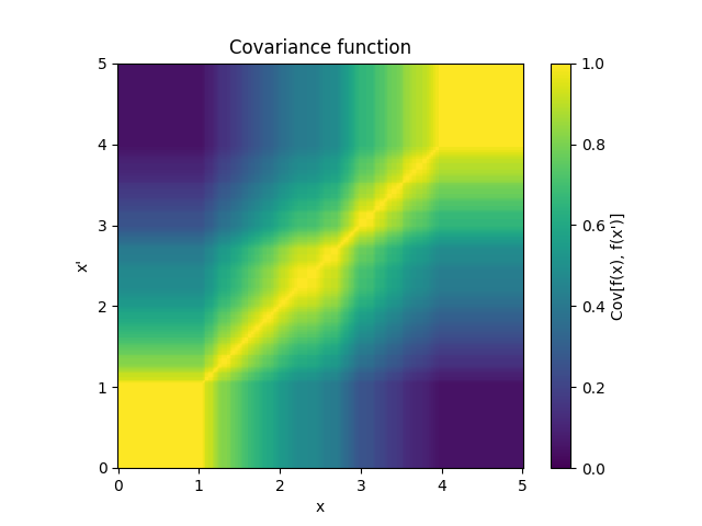
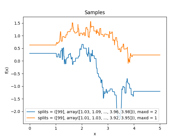
- class lsqfitgp.BART(**kw)[source]
BART kernel.
Good default parameters:
maxd=4, reset=2ifalphaandbetaare kept fixed at the default values,maxd=10, reset=[2,4,6,8]otherwise. Derivatives are faster with forward autodiff.- Parameters:
- x, yarrays
Input points. The array type can be structured, in which case every leaf field represents a dimension; or unstructured, which specifies a single dimension.
- alpha, betascalar
The parameters of the branching probability.
- maxdint
The maximum depth of the trees.
- splitspair of arrays
The first is an int (p,) array containing the number of splitting points along each dimension, the second has shape (n, p) and contains the sorted splitting points in each column, filled with high values after the length. Use
BART.splits_from_coordto produce them.- gammascalar or str
Interpolation coefficient in [0, 1] between a lower and a upper bound on the infinite maxd limit, or a string ‘auto’ indicating to use a formula which depends on alpha, beta, maxd and the number of covariates, empirically calibrated on maxd from 1 to 3. Default 1 (upper bound).
- pnt(maxd + 1,) array, optional
Nontermination probabilities at depths 0…maxd. If specified,
alpha,betaandmaxdare ignored.- interceptbool, default True
The correlation is in [1 - alpha, 1] (or [1 - pnt[0], 1] when using pnt). If intercept=False, it is rescaled to [0, 1].
- weights(p,) array, optional
Unnormalized selection probabilities for the covariate axes. If not specified, all axes have the same probability to be selected for splitting.
- resetint or sequence of int, optional
List of depths at which the recursion is reset, in the sense that the function value at a reset depth is evaluated on the initial inputs for all recursion paths, instead of the modified input handed down by the recursion. Default none.
- indicesbool, default False
If False, the inputs
x,yrepresent coordinate values. If True, they are taken to be already the indices of the points in the splitting grid, as can be obtained withBART.indices_from_coord.
Methods
Generate splitting points from data.
indices_from_coord(x, splits)Convert coordinates to indices w.r.t.
correlation(splitsbefore_or_totalsplits, ...)Compute the BART prior correlation between two points.
Notes
This is the covariance function of the latent mean prior of BART (Bayesian Additive Regression Trees) [1] with an upper bound \(D\) on the depth of the trees. This prior is the distribution of the function
\[f(\mathbf x) = \lim_{m\to\infty} \sum_{j=1}^m g(\mathbf x; T_j, M_j),\]where each \(g(\mathbf x; T_j, M_j)\) is a decision tree evaluated at \(\mathbf x\), with structure \(T_j\) and leaf values \(M_j\). The trees are i.i.d., with the following distribution for \(T_j\): for a node at depth \(d\), with \(d = 0\) for the root, the probability of not being a leaf, conditional on its existence and its ancestors only, is
\[P_d = \alpha (1+d)^{-\beta}, \quad \alpha \in [0, 1], \quad \beta \ge 0.\]For a non-leaf node, conditional on existence and ancestors, the splitting variable has uniform distribution amongst the variables with any splitting points not used by ancestors, and the splitting point has uniform distribution amongst the available ones. The splitting points are fixed, tipically from the data.
The distribution of leaves \(M_j\) is i.i.d. Normal with variance \(1/m\), such that \(f(x)\) has variance 1. In the limit \(m\to\infty\), the distribution of \(f(x)\) becomes a Gaussian process.
Since the trees are independent, the covariance function can be computed for a single tree. Consider two coordinates \(x\) and \(y\), with \(x \le y\). Let \(n^-\), \(n^0\) and \(n^+\) be the number of splitting points respectively before \(x\), between \(x\), \(y\) and after \(y\). Next, define \(\mathbf n^-\), \(\mathbf n^0\) and \(\mathbf n^+\) as the vectors of such quantities for each dimension, with a total of \(p\) dimensions, and \(\mathbf n = \mathbf n^- + \mathbf n^0 + \mathbf n^+\). Then the covariance function can be written recursively as
\[\begin{split}\newcommand{\nvecs}{\mathbf n^-, \mathbf n^0, \mathbf n^+} k(\mathbf x, \mathbf y) &= k_0(\nvecs), \\ k_D(\nvecs) &= 1 - (1 - \gamma) P_D, \quad \mathbf n^0 \ne \mathbf 0, \\ k_d(\mathbf 0, \mathbf 0, \mathbf 0) &= 1, \\ k_d(\nvecs) &= 1 - P_d \Bigg(1 - \frac1{W(\mathbf n)} \sum_{\substack{i=1 \\ n_i\ne 0}}^p \frac{w_i}{n_i} \Bigg( \\ &\qquad \sum_{k=0}^{n^-_i - 1} k_{d+1}(\mathbf n^-_{n^-_i=k}, \mathbf n^0, \mathbf n^+) + {} \\ &\qquad \sum_{k=0}^{n^+_i - 1} k_{d+1}(\mathbf n^-, \mathbf n^0, \mathbf n^+_{n^+_i=k}) \Bigg) \Bigg), \quad d < D, \\ W(\mathbf n) &= \sum_{\substack{i=1 \\ n_i\ne 0}}^p w_i.\end{split}\]The introduction of a maximum depth \(D\) is necessary for computational feasibility. As \(D\) increases, the result converges to the one without depth limit. For \(D \le 2\) (the default value), the covariance is implemented in closed form and takes \(O(p)\) to compute. For \(D > 2\), the computational complexity grows exponentially as \(O(p(\bar np)^{D-2})\), where \(\bar n\) is the average number of splitting points along a dimension.
In the maximum allowed depth is 1, i.e., either \(D = 1\) or \(\beta\to\infty\), the kernel assumes the simple form
\[\begin{split}k(\mathbf x, \mathbf y) &= 1 - P_0 \left( 1 - Q + \frac Q{W(\mathbf n)} \sum_{\substack{i=1 \\ n_i\ne 0}}^p w_i \frac{n^0_i}{n_i} \right), \\ Q &= \begin{cases} 1 - (1 - \gamma) P_1 & \mathbf n^0 \ne \mathbf 0, \\ 1 & \mathbf n^0 = \mathbf 0, \end{cases}\end{split}\]which is separable along dimensions, i.e., it has no interactions.
References
[1]Hugh A. Chipman, Edward I. George, Robert E. McCulloch “BART: Bayesian additive regression trees,” The Annals of Applied Statistics, Ann. Appl. Stat. 4(1), 266-298, (March 2010).
- classmethod correlation(splitsbefore_or_totalsplits, splitsbetween_or_index1, splitsafter_or_index2, *, alpha=0.95, beta=2, gamma=1, maxd=2, debug=False, pnt=None, intercept=True, weights=None, reset=None, altinput=False)[source]
Compute the BART prior correlation between two points.
Apart from arguments
maxd,debugandreset, this method is fully vectorized.- Parameters:
- splitsbefore_or_totalsplitsint (p,) array
The number of splitting points less than the two points, separately along each coordinate, or the total number of splits if
altinput.- splitsbetween_or_index1int (p,) array
The number of splitting points between the two points, separately along each coordinate, or the index in the splitting bins of the first point if
altinput, where 0 means to the left of the leftmost splitting point.- splitsafter_or_index2int (p,) array
The number of splitting points greater than the two points, separately along each coordinate, or the index in the splitting bins of the second point if
altinput.- debugbool
If True, disable shortcuts in the tree recursion. Default False.
- altinputbool
If True, take as input the indices in the splitting bins of the points instead of the counts of splitting points separating them, and use a different implementation optimized for that case. Default False. The
BARTkernel usesaltinput=True.- Other parameters
See
BART.
- Returns:
- corrscalar
The prior correlation.
- classmethod indices_from_coord(x, splits)[source]
Convert coordinates to indices w.r.t. splitting points.
- Parameters:
- xarray of numbers
The coordinates. Can be passed in two formats: 1) a structured array where each leaf field represents a dimension, 2) a normal array where the last axis runs over dimensions. In the structured case, each index in any shaped field is a different dimension.
- splitspair of arrays
The first is an int (p,) array containing the number of splitting points along each dimension, the second has shape (n, p) and contains the sorted splitting points in each column, filled with high values after the length.
- Returns:
- ixint array
An array with the same shape as
x, unlessxis a structured array, in which case the last axis ofixis the flattened version of the structured type.ixcontains indices mappingxto positions between splitting points along each coordinate, with the following convention: index 0 means before the first split, index i > 0 means between split i - 1 and split i.
- classmethod splits_from_coord(x)[source]
Generate splitting points from data.
- Parameters:
- xarray of numbers
The data. Can be passed in two formats: 1) a structured array where each leaf field represents a dimension, 2) a normal array where the last axis runs over dimensions. In the structured case, each index in any shaped field is a different dimension.
- Returns:
- lengthint (p,) array
The number of splitting points along each of
pdimensions.- splits(n, p) array
Each column contains the sorted splitting points along a dimension. The splitting points are the midpoints between consecutive values appearing in
xfor that dimension. Columnsplits[:, i]contains splitting points only up tolength[i], while afterward it is filled with a very large value.
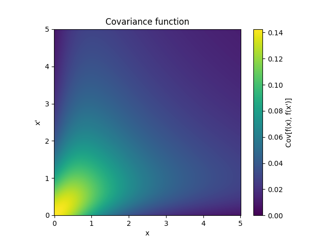
- class lsqfitgp.BagOfWords(**kw)[source]
Bag of words kernel.
\[\begin{split}k(x, y) &= \sum_{w \in \text{words}} c_w(x) c_w(y), \\ c_w(x) &= \text{number of times word $w$ appears in $x$}\end{split}\]The words are defined as non-empty substrings delimited by spaces or one of the following punctuation characters: ! « » “ “ ” ‘ ’ / ( ) ‘ ? ¡ ¿ „ ‚ < > , ; . : - – —.
Reference: Rasmussen and Williams (2006, p. 100).
- class lsqfitgp.Bessel(**kw)[source]
Bessel kernel.
\[k(r) = \Gamma(\nu + 1) 2^\nu (sr)^{-\nu} J_{\nu}(sr), \quad s = 2 + \nu / 2, \quad \nu \ge 0,\]where \(s\) is a crude estimate of the half width at half maximum of \(J_\nu\). Can be used in up to \(2(\lfloor\nu\rfloor + 1)\) dimensions and derived up to \(\lfloor\nu/2\rfloor\) times.
Reference: Rasmussen and Williams (2006, p. 89).
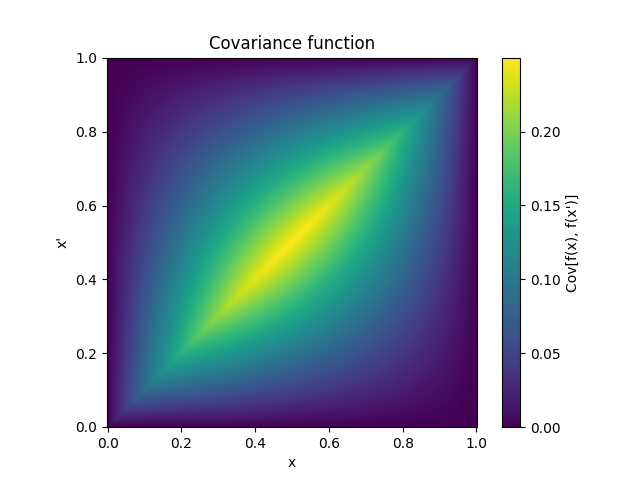
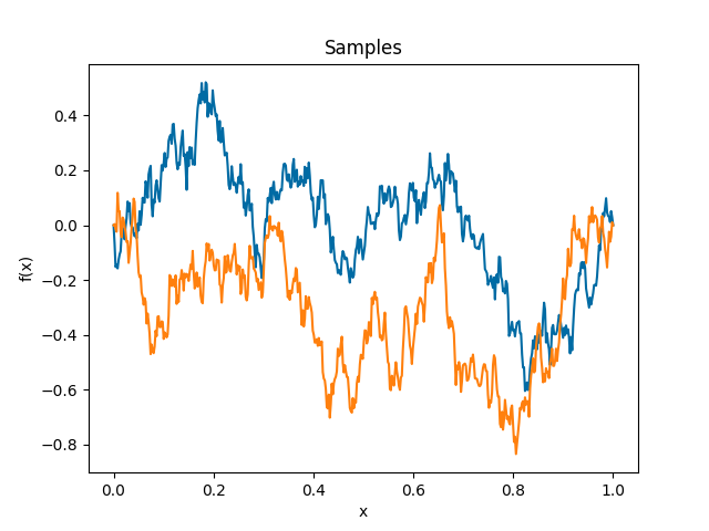
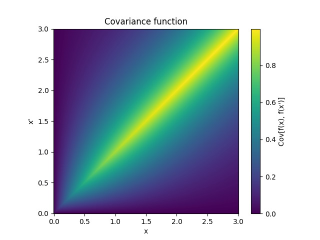
- class lsqfitgp.BrownianBridge(**kw)[source]
Brownian bridge kernel.
\[k(x, y) = \min(x, y) - xy, \quad x, y \in [0, 1]\]It is a Wiener process conditioned on being zero at x = 1.
- class lsqfitgp.Categorical(**kw)[source]
Categorical kernel.
\[k(x, y) = \texttt{cov}[x, y]\]A kernel over integers from 0 to N-1. The parameter
covis the covariance matrix of the values.
- class lsqfitgp.Cauchy(**kw)[source]
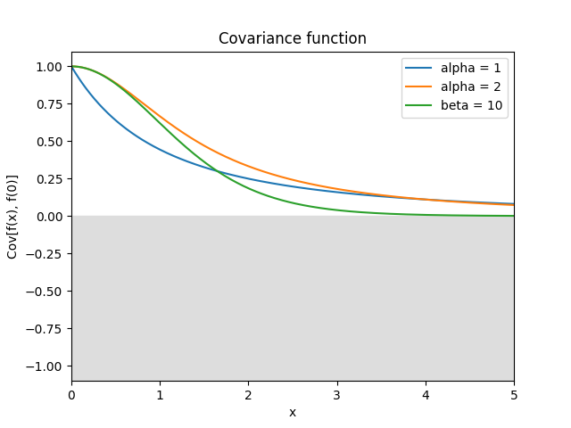
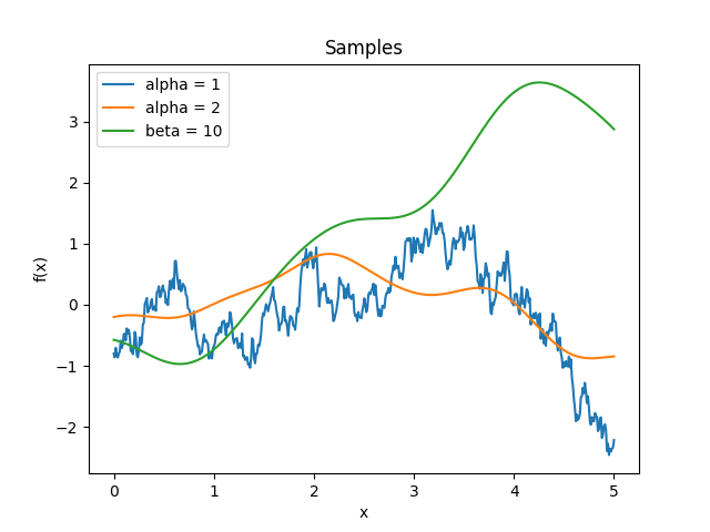
Generalized Cauchy kernel.
\[k(r) = \left(1 + \frac{r^\alpha}{\beta} \right)^{-\beta/\alpha}, \quad \alpha \in (0, 2], \beta > 0.\]In the geostatistics literature, the case \(\alpha=2\) and \(\beta=2\) (default) is known as the Cauchy kernel. In the machine learning literature, the case \(\alpha=2\) (for any \(\beta\)) is known as the rational quadratic kernel. For \(\beta\to\infty\) it is equivalent to
GammaExp(gamma=alpha, scale=alpha ** (1/alpha)), while for \(\beta\to 0\) toConstant. It is smooth only for \(\alpha=2\).References: Gneiting and Schlather (2004, p. 273), Rasmussen and Williams (2006, p. 86).
- class lsqfitgp.CausalExpQuad(**kw)[source]
Causal exponential quadratic kernel.
\[k(r) = \big(1 - \operatorname{erf}(\alpha r/4)\big) \exp\left(-\frac12 r^2 \right)\]
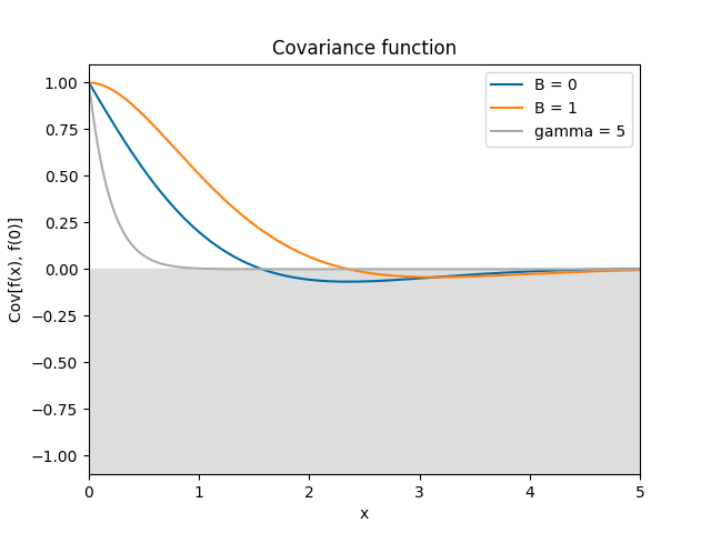
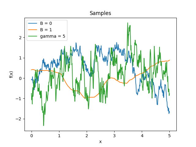
- class lsqfitgp.Celerite(**kw)[source]
Celerite kernel.
\[k(\Delta) = \exp(-\gamma|\Delta|) \big( \cos(\Delta) + B \sin(|\Delta|) \big)\]This is the covariance function of an AR(2) process with complex roots. The parameters must satisfy the condition \(|B| \le \gamma\). For \(B = \gamma\) it is equivalent to the
Harmonickernel with \(\eta Q = 1/B, Q > 1\), and it is derivable.Reference: Daniel Foreman-Mackey, Eric Agol, Sivaram Ambikasaran, and Ruth Angus: Fast and Scalable Gaussian Process Modeling With Applications To Astronomical Time Series.
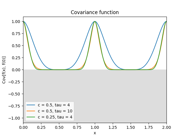
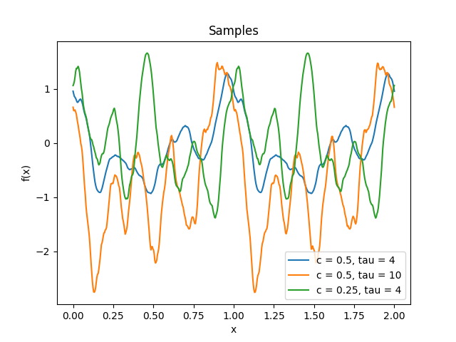
- class lsqfitgp.Circular(**kw)[source]
Circular kernel.
\[\begin{split}k(x, y) &= W_c(d_{\text{geo}}(x, y)), \\ W_c(t) &= \left(1 + \tau\frac tc\right) \left(1 - \frac tc\right)^\tau_+, \quad c \in (0, 1/2], \tau \ge 4, \\ d_{\text{geo}}(x, y) &= \arccos\cos(2\pi(x-y)).\end{split}\]It is a stationary periodic kernel with period 1.
Reference: Padonou and Roustant (2016).
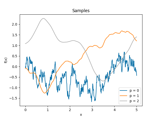
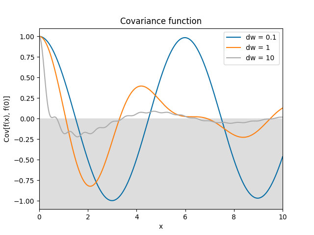
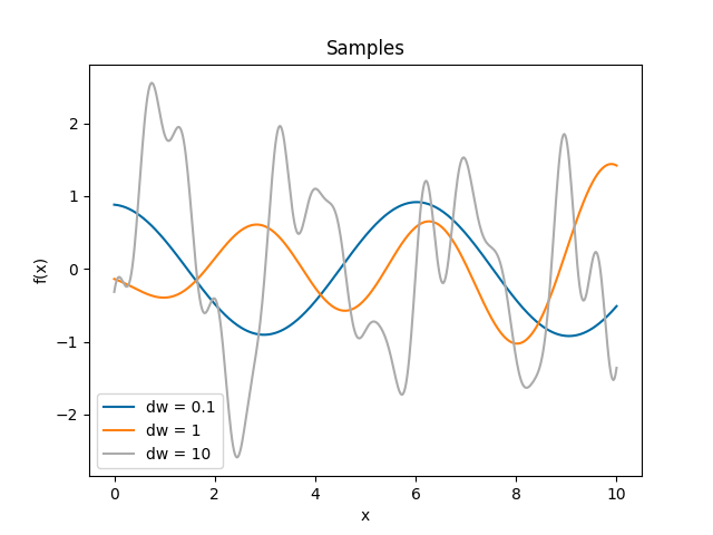
- class lsqfitgp.Color(**kw)[source]
Colored noise kernel.
\[\begin{split}k(\Delta) &= (n-1) \Re E_n(-i\Delta) = \\ &= (n-1) \int_1^\infty \mathrm d\omega \frac{\cos(\omega\Delta)}{\omega^n}, \quad n \in \mathbb N, n \ge 2.\end{split}\]A process with power spectrum \(1/\omega^n\) truncated below \(\omega = 1\). \(\omega\) is the angular frequency \(\omega = 2\pi f\). Derivable \(\lfloor n/2 \rfloor - 1\) times.
- class lsqfitgp.Constant(**kw)[source]
Constant kernel.
\[k(x, y) = 1\]This means that all points are completely correlated, thus it is equivalent to fitting with a horizontal line. This can be seen also by observing that 1 = 1 x 1.
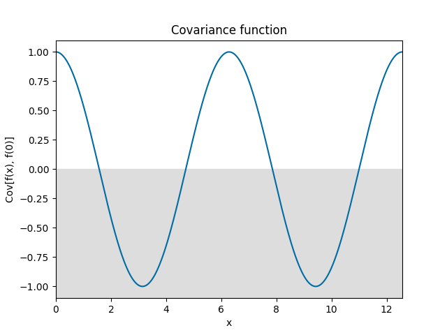
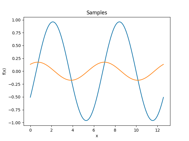
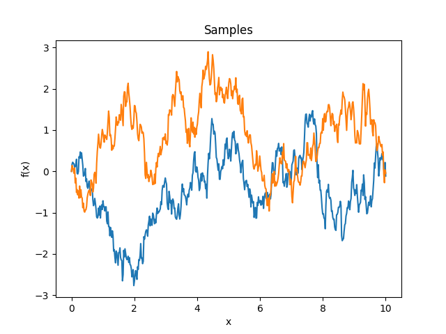
- class lsqfitgp.Cos(**kw)[source]
Cosine kernel.
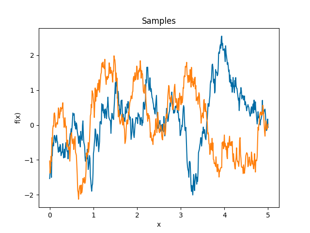
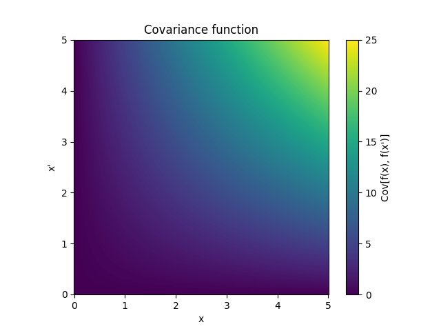
\[k(\Delta) = \cos(\Delta) = \cos x \cos y + \sin x \sin y\]Samples from this kernel are harmonic functions. It can be multiplied with another kernel to introduce anticorrelations.
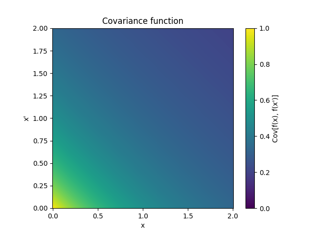
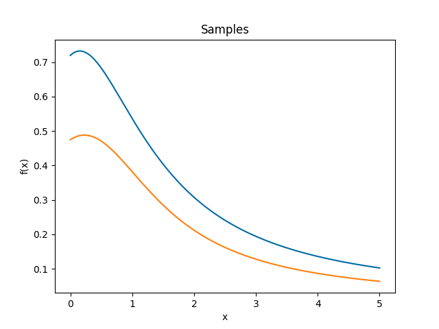
- class lsqfitgp.Decaying(**kw)[source]
Decaying kernel.
\[k(x, y) = \frac{1}{(1 + x + y)^\alpha}, \quad x, y, \alpha \ge 0\]Reference: Swersky, Snoek and Adams (2014).

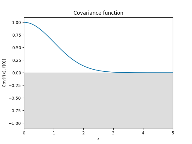
- class lsqfitgp.ExpQuad(**kw)[source]
Exponential quadratic kernel.
\[k(r) = \exp \left( -\frac 12 r^2 \right)\]It is smooth and has a strict typical lengthscale, i.e., oscillations are strongly suppressed under a certain wavelength, and correlations are strongly suppressed over a certain distance.
Reference: Rasmussen and Williams (2006, p. 83).
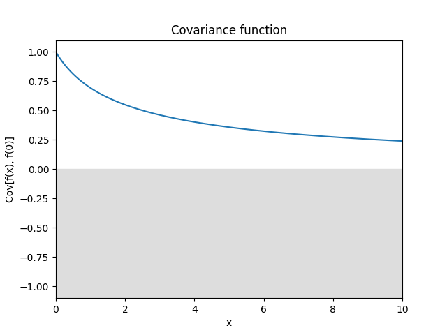
- class lsqfitgp.Expon(**kw)[source]
Exponential kernel.
\[k(\Delta) = \exp(-|\Delta|)\]In 1D it is equivalent to the Matérn 1/2 kernel, however in more dimensions it acts separately while the Matérn kernel is isotropic.
Reference: Rasmussen and Williams (2006, p. 85).
- class lsqfitgp.FracBrownian(**kw)[source]
Bifractional Brownian motion kernel.
\[k(x, y) = \frac 1{2^K} \big( (|x|^{2H} + |y|^{2H})^K - |x-y|^{2HK} \big), \quad H, K \in (0, 1]\]For \(H = 1/2\) (default) it is the Wiener kernel. For \(H \in (0, 1/2)\) the increments are anticorrelated (strong oscillation), for \(H \in (1/2, 1]\) the increments are correlated (tends to keep a slope).
Reference: Houdré and Villa (2003).
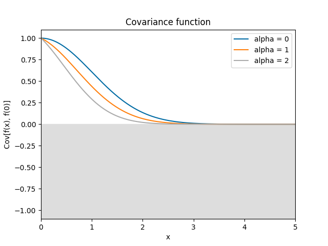
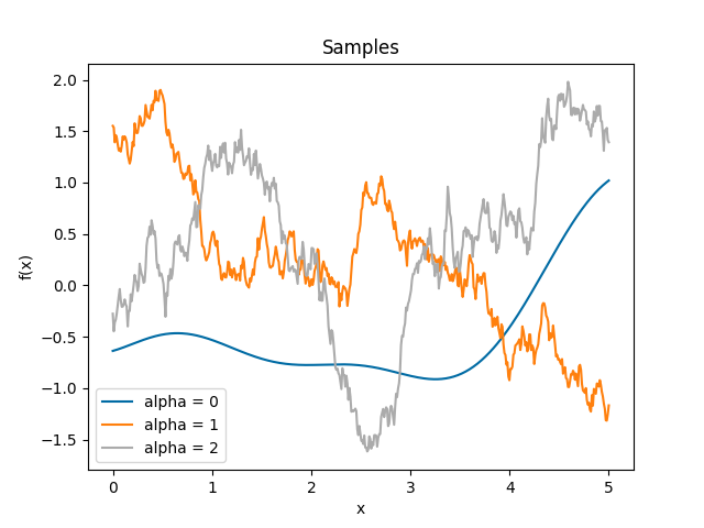
- class lsqfitgp.GammaExp(**kw)[source]
Gamma exponential kernel.
\[k(r) = \exp(-r^\gamma), \quad \gamma \in (0, 2]\]For \(\gamma = 2\) it is the squared exponential kernel, for \(\gamma = 1\) (default) it is the Matérn 1/2 kernel, for \(\gamma \to 0\) it tends to white noise plus a constant. The process is differentiable only for \(\gamma = 2\), however as \(\gamma\) gets closer to 2 the variance of the non-derivable component goes to zero.
Reference: Rasmussen and Williams (2006, p. 86).
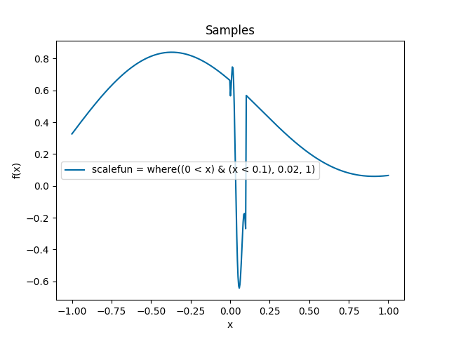
- class lsqfitgp.Gibbs(**kw)[source]
Gibbs kernel.
\[k(x, y) = \sqrt{ \frac {2 s(x) s(y)} {s(x)^2 + s(y)^2} } \exp \left( -\frac {(x - y)^2} {s(x)^2 + s(y)^2} \right), \quad s = \texttt{scalefun}.\]Kernel which in some sense is like a Gaussian kernel where the scale changes at every point. The scale is computed by the parameter
scalefunwhich must be a callable taking the x array and returning a scale for each point. By defaultscalefunreturns 1 so it is a Gaussian kernel.Consider that the default parameter
scaleacts beforescalefun, so for example ifscalefun(x) = xthenscalehas no effect. You should include all rescalings inscalefunto avoid surprises.Reference: Rasmussen and Williams (2006, p. 93).
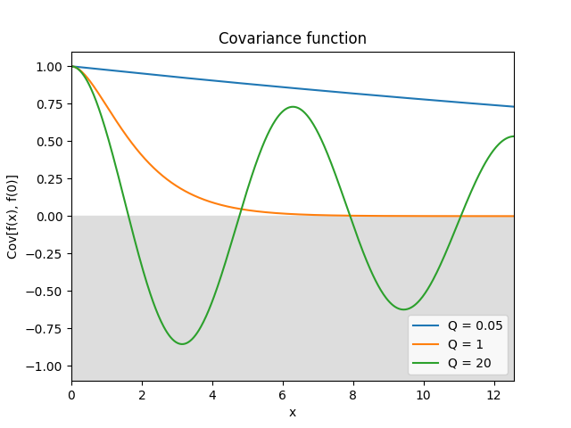
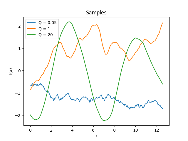
- class lsqfitgp.Harmonic(**kw)[source]
Damped stochastically driven harmonic oscillator kernel.
\[\begin{split}k(\Delta) = \exp\left( -\frac {|\Delta|} {Q} \right) \begin{cases} \cosh(\eta\Delta) + \sinh(\eta|\Delta|) / (\eta Q) & 0 < Q < 1 \\ 1 + |\Delta| & Q = 1 \\ \cos(\eta\Delta) + \sin(\eta|\Delta|) / (\eta Q) & Q > 1, \end{cases}\end{split}\]where \(\eta = \sqrt{|1 - 1/Q^2|}\).
The process is the solution to the stochastic differential equation
\[f''(x) + 2/Q f'(x) + f(x) = w(x),\]where \(w\) is white noise.
The parameter \(Q\) is the quality factor, i.e., the ratio between the energy stored in the oscillator and the energy lost in each cycle due to damping. The angular frequency is 1, i.e., the period is 2π. The process is derivable one time.
In 1D, for \(Q = 1\) (default) and
scale=sqrt(1/3), it is the Matérn 3/2 kernel.Reference: Daniel Foreman-Mackey, Eric Agol, Sivaram Ambikasaran, and Ruth Angus: Fast and Scalable Gaussian Process Modeling With Applications To Astronomical Time Series.
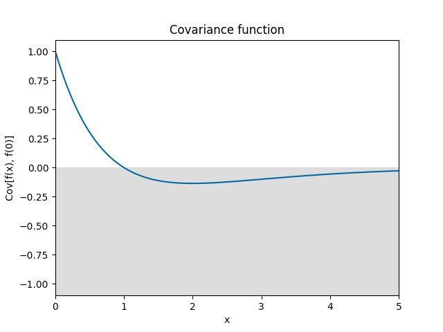
- class lsqfitgp.HoleEffect(**kw)[source]
Hole effect kernel.
\[k(\Delta) = (1 - \Delta) \exp(-\Delta)\]Reference: Dietrich and Newsam (1997, p. 1096).
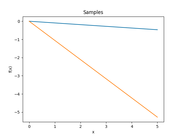
- class lsqfitgp.Linear(**kw)[source]
Dot product kernel.
\[k(x, y) = x \cdot y = \sum_i x_i y_i\]In 1D it is equivalent to fitting with a line passing by the origin.
Reference: Rasmussen and Williams (2006, p. 89).
- class lsqfitgp.MA(**kw)[source]
Discrete moving average kernel.
\[k(\Delta) = \sum_{k=|\Delta|}^{n-1} w_k w_{k-|\Delta|}, \quad \mathbf w = (w_0, \ldots, w_{n-1}).\]The inputs must be integers. It is the autocovariance function of a moving average with weights \(\mathbf w\) applied to white noise:
\[\begin{split}k(i, j) &= \operatorname{Cov}[y_i, y_j], \\ y_i &= \sum_{k=0}^{n-1} w_k \epsilon_{i-k}, \\ \operatorname{Cov}[\epsilon_i,\epsilon_j] &= \delta_{ij}.\end{split}\]If
norm=True, the variance is normalized to 1, which amounts to normalizing \(\mathbf w\) to unit length.
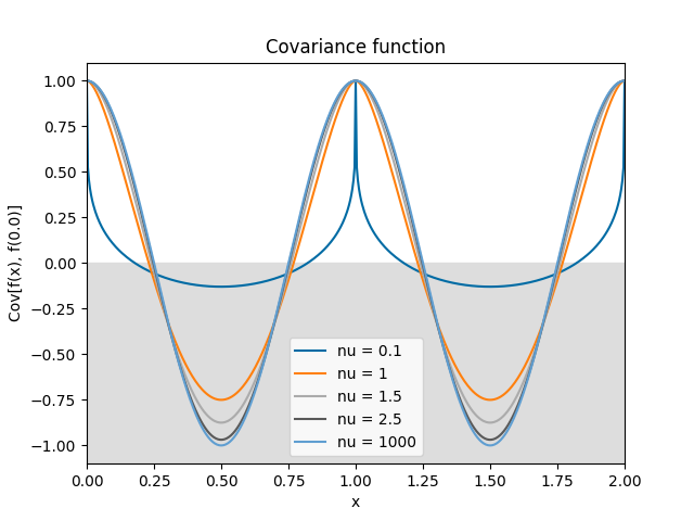
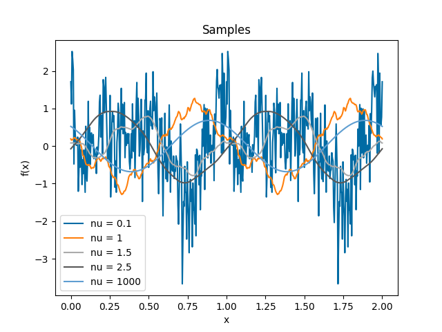
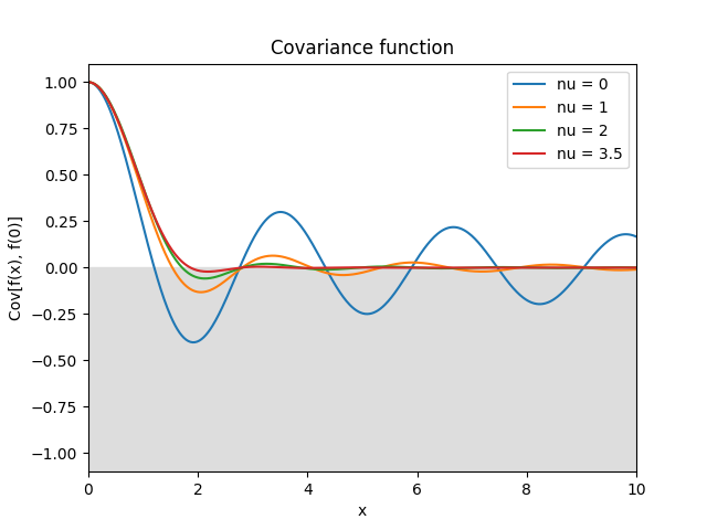
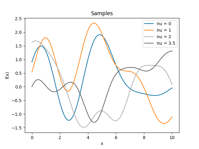
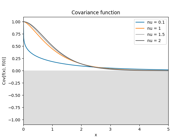
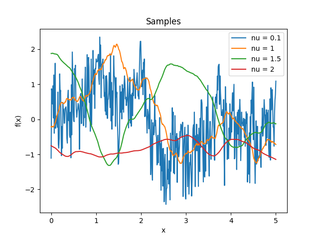
- class lsqfitgp.Matern(**kw)[source]
Matérn kernel of real order.
\[k(r) = \frac {2^{1-\nu}} {\Gamma(\nu)} x^\nu K_\nu(x), \quad \nu \ge 0, \quad x = \sqrt{2\nu} r\]The process is \(\lceil\nu\rceil-1\) times derivable: so for \(0 \le \nu \le 1\) it is not derivable, for \(1 < \nu \le 2\) it is derivable but has not a second derivative, etc. The highest derivative is (Lipschitz) continuous iff \(\nu\bmod 1 \ge 1/2\).
Reference: Rasmussen and Williams (2006, p. 84).
- class lsqfitgp.Maternp(**kw)[source]
Matérn kernel of half-integer order.
\[\begin{split}k(r) &= \frac {2^{1-\nu}} {\Gamma(\nu)} x^\nu K_\nu(x) = \\ &= \exp(-x) \frac{p!}{(2p)!} \sum_{i=0}^p \frac{(p+i)!}{i!(p-i)!} (2x)^{p-i} \\ \nu &= p + 1/2, p \in \mathbb N, x = \sqrt{2\nu} r\end{split}\]The degree of derivability is \(p\).
Reference: Rasmussen and Williams (2006, p. 85).
- class lsqfitgp.NNKernel(**kw)[source]
Neural network kernel.
\[k(x, y) = \frac 2 \pi \arcsin \left( \frac { 2 (q + x \cdot y) }{ (1 + 2 (q + x \cdot x)) (1 + 2 (q + y \cdot y)) } \right), \quad q = \texttt{sigma0}^2\]Kernel which is equivalent to a neural network with one infinite hidden layer with Gaussian priors on the weights and error function response. In other words, you can think of the process as a superposition of sigmoids where
sigma0sets the dispersion of the centers of the sigmoids.Reference: Rasmussen and Williams (2006, p. 90).
- class lsqfitgp.OrnsteinUhlenbeck(**kw)[source]
Ornstein-Uhlenbeck process kernel.
\[k(x, y) = \exp(-|x - y|) - \exp(-(x + y)), \quad x, y \ge 0\]It is a random walk plus a negative feedback term that keeps the asymptotical variance constant. It is asymptotically stationary; often the name “Ornstein-Uhlenbeck” is given to the stationary part only, which here is provided as
Expon.
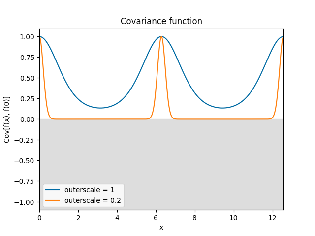
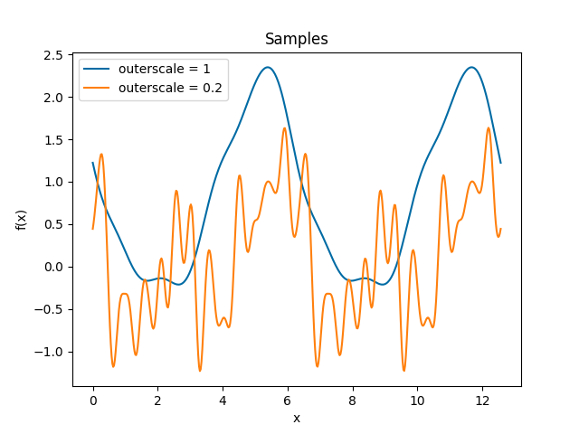
- class lsqfitgp.Periodic(**kw)[source]
Periodic Gaussian kernel.
\[k(\Delta) = \exp \left( -2 \left( \frac {\sin(\Delta / 2)} {\texttt{outerscale}} \right)^2 \right)\]A Gaussian kernel over a transformed periodic space. It represents a periodic process. The usual
scaleparameter sets the period, with the defaultscale=1giving a period of 2π, whileouterscalesets the length scale of the correlations.Reference: Rasmussen and Williams (2006, p. 92).
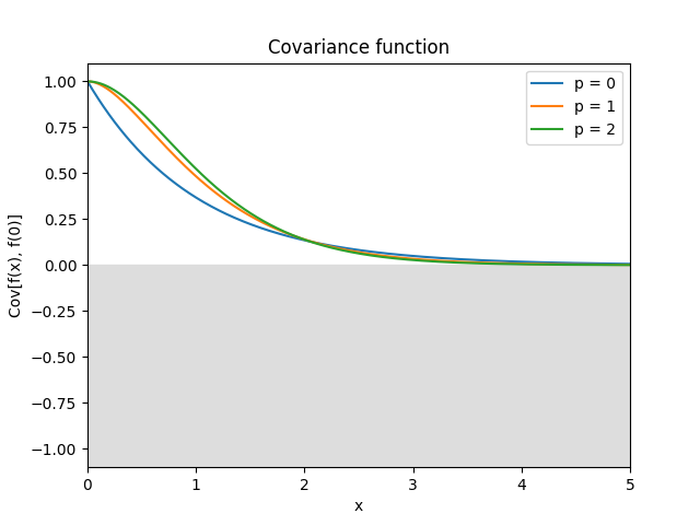
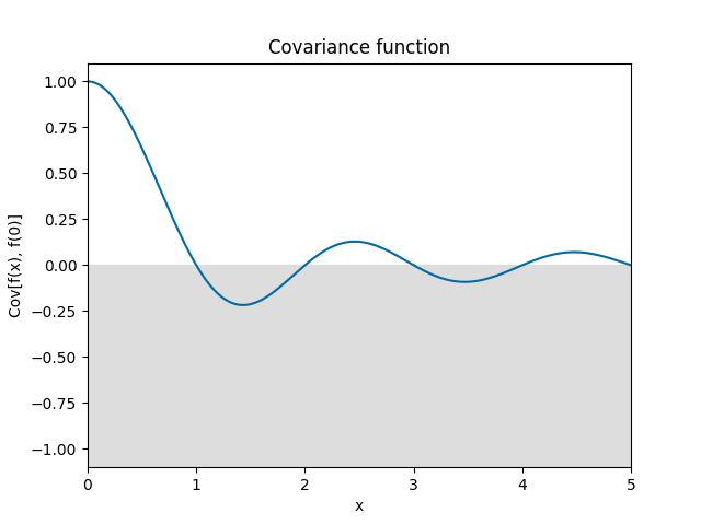
- class lsqfitgp.Pink(**kw)[source]
Pink noise kernel.
\[\begin{split}k(\Delta) &= \frac 1 {\log(1 + \delta\omega)} \int_1^{1+\delta\omega} \mathrm d\omega \frac{\cos(\omega\Delta)}\omega = \\ &= \frac { \operatorname{Ci}(\Delta (1 + \delta\omega)) - \operatorname{Ci}(\Delta) } {\log(1 + \delta\omega)}\end{split}\]A process with power spectrum \(1/\omega\) truncated between 1 and \(1 + \delta\omega\). \(\omega\) is the angular frequency \(\omega = 2\pi f\). In the limit \(\delta\omega\to\infty\) it becomes white noise. Derivable one time.
- class lsqfitgp.Rescaling(**kw)[source]
Outer product kernel.
\[k(x, y) = \texttt{stdfun}(x) \texttt{stdfun}(y)\]A totally correlated kernel with arbitrary variance. Parameter
stdfunmust be a function that takesxoryand computes the standard deviation at the point. It can yield negative values; points with the same sign ofstdfunwill be totally correlated, points with different sign will be totally anticorrelated. Use this kernel to modulate the variance of other kernels. By defaultstdfunreturns a constant, so it is equivalent toConstant.
- class lsqfitgp.Sinc(**kw)[source]
Sinc kernel.
\[k(\Delta) = \operatorname{sinc}(\Delta) = \frac{\sin(\pi\Delta)}{\pi\Delta}.\]Reference: Tobar (2019).
- class lsqfitgp.StationaryFracBrownian(**kw)[source]
Stationary fractional Brownian motion kernel.
\[k(\Delta) = \frac 12 (|\Delta+1|^{2H} + |\Delta-1|^{2H} - 2|\Delta|^{2H}), \quad H \in (0, 1]\]Reference: Gneiting and Schlather (2006, p. 272).
- class lsqfitgp.Taylor(**kw)[source]
Exponential-like power series kernel.
\[k(x, y) = \sum_{k=0}^\infty \frac {x^k}{k!} \frac {y^k}{k!} = I_0(2 \sqrt{xy})\]It is equivalent to fitting with a Taylor series expansion in zero with independent priors on the coefficients k with mean zero and standard deviation 1/k!.
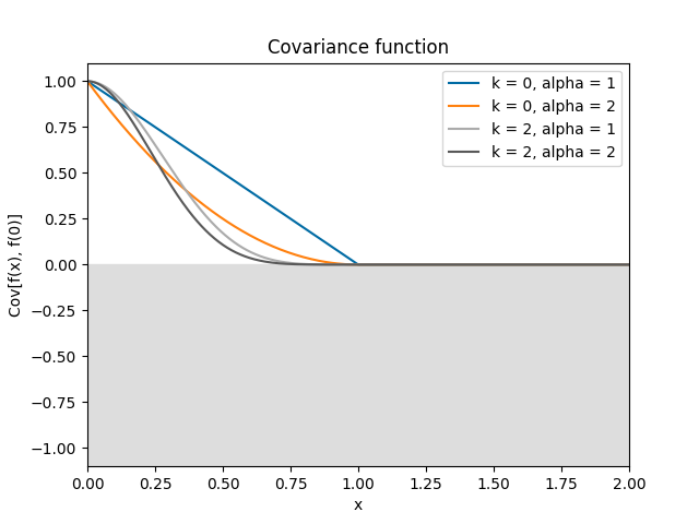
- class lsqfitgp.Wendland(**kw)[source]
Wendland kernel.
\[\begin{split}k(r) &= \frac1{B(2k+1,\nu)} \int_r^\infty \mathrm du\, (u^2 - r^2)^k (1 - u)_+^{\nu-1}, \\ \quad k &\in \mathbb N,\ \nu = k + \alpha,\ \alpha \ge 1.\end{split}\]An isotropic kernel with finite support. The covariance is nonzero only when the distance between the points is less than 1. Parameter \(k \in \{0, 1, 2, 3\}\) sets the differentiability, while the maximum dimensionality the kernel can be used in is \(\lfloor 2\alpha-1 \rfloor\). Default is \(k = 0\) (non derivable), \(\alpha = 1\) (can be used only in 1D).
Reference: Gneiting (2002), Wendland (2004, p. 128), Rasmussen and Williams (2006, p. 87), Porcu, Furrer and Nychka (2020, p. 4).
- class lsqfitgp.White(**kw)[source]
White noise kernel.
\[\begin{split}k(x, y) = \begin{cases} 1 & x = y \\ 0 & x \neq y \end{cases}\end{split}\]
- class lsqfitgp.Wiener(**kw)[source]
Wiener kernel.
\[k(x, y) = \min(x, y), \quad x, y > 0\]A kernel representing a non-differentiable random walk starting at 0.
Reference: Rasmussen and Williams (2006, p. 94).
- class lsqfitgp.WienerIntegral(**kw)[source]
Kernel for a process whose derivative is a Wiener process.
\[k(x, y) = \frac 12 a^2 \left(b - \frac a3 \right), \quad a = \min(x, y), b = \max(x, y)\]
- class lsqfitgp.Zeta(**kw)[source]
Zeta kernel.
\[\begin{split}k(\Delta) &= \frac{\Re F(\Delta, s)}{\zeta(s)} = \qquad (s = 1 + 2 \nu, \quad \nu \ge 0) \\ &= \frac1{\zeta(s)} \sum_{k=1}^\infty \frac {\cos(2\pi k\Delta)} {k^s} = \\ &= -(-1)^{s/2} \frac {(2\pi)^s} {2s!} \frac {\tilde B_s(\Delta)} {\zeta(s)} \quad \text{for even integer $s$.}\end{split}\]It is equivalent to fitting with a Fourier series of period 1 with independent priors on the coefficients with mean zero and variance \(1/(\zeta(s)k^s)\) for the \(k\)-th term. Analogously to
Matern, the process is \(\lceil\nu\rceil - 1\) times derivable, and the highest derivative is continuous iff \(\nu\bmod 1 \ge 1/2\).The \(k = 0\) term is not included in the summation, so the mean of the process over one period is forced to be zero.
Reference: Petrillo (2022).