10. Splitting components

In More on kernels we saw an example where we summed two ExpQuad kernels with different scale, and the result effectively looked like the sum of two processes, because the kernel of a sum of processes is the sum of their kernels.

When summing processes it is useful to get the fit result separately for each component. In lsqfitgp there’s not a specific tool for this because it can be implemented using kernel tricks, multidimensional input and transformations.

Let’s see. We first generate some data:

import numpy as np
import lsqfitgp as lgp
import gvar
from matplotlib import pyplot as plt

gp = lgp.GP(10 * lgp.ExpQuad(scale=10) + lgp.ExpQuad(scale=1))

x = np.linspace(-10, 10, 21)
gp.addx(x, 'pinguini')

prior = gp.prior('pinguini')
y = gvar.sample(prior)

fig, ax = plt.subplots(num='lsqfitgp example')

ax.plot(x, y, '.k')

fig.savefig('components1.png')

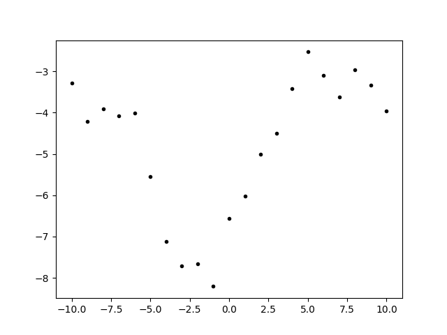
We made a mixture of two exponential quadratics and took a sample from the prior as data. Generating fake data from the prior is a good way to make sure that the fit will make sense with the data.

Now we setup a fit with an additional integer input dimension that indicates the component, similarly to what we did in Multidimensional output:

xtype = np.dtype([
    ('x'   , float),
    ('comp', int  ),
])
xcomp = np.empty((2, len(x)), xtype)
xcomp['x'   ] = x  # broadcasting aligns the last axes
xcomp['comp'] = np.array([0, 1])[:, None]

We need to make a kernel that changes based on the value in the 'comp' field. We can do that by using a Rescaling that acts on 'comp':

kernel1 = 10 * lgp.ExpQuad(scale=10)
kernel2 = lgp.ExpQuad(scale=1)

kernel = kernel1 * lgp.Rescaling(stdfun=lambda x: x['comp'] == 0)
kernel += kernel2 * lgp.Rescaling(stdfun=lambda x: x['comp'] == 1)

gp = lgp.GP(kernel)

The boolean operation in the stdfun argument returns 0 or 1, and since stdfun is called on both arguments of the kernel, each component is nonzero only when acting on two points which have the same 'comp'.

Now we add separately the two components and sum them with addtransf():

gp.addx(xcomp[0], 'longscale')
gp.addx(xcomp[1], 'shortscale')
gp.addtransf({'shortscale': 1, 'longscale': 1}, 'sum')

We can now proceed as usual to get the posterior on other points:

xplot = np.empty((2, 200), dtype=xtype)
xplot['x'] = np.linspace(-10, 10, xplot.shape[1])
xplot['comp'] = np.array([0, 1])[:, None]

gp.addx(xplot[0], 'longscale_plot')
gp.addx(xplot[1], 'shortscale_plot')
gp.addtransf({'longscale_plot': 1, 'shortscale_plot': 1}, 'sum_plot')

post = gp.predfromdata({'sum': y})

ax.cla()

for sample in gvar.raniter(post, 2):
    line, = ax.plot(xplot[0]['x'], sample['sum_plot'])
    color = line.get_color()
    ax.plot(xplot[0]['x'], sample['longscale_plot'], '--', color=color)
    ax.plot(xplot[0]['x'], sample['shortscale_plot'], ':', color=color)

ax.plot(x, y, '.k')

fig.savefig('components2.png')

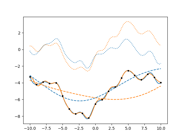
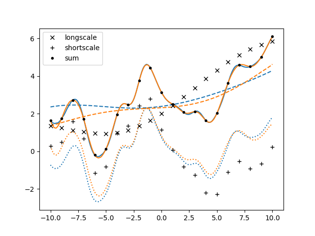
It’s interesting to note that the uncertainty on the individual components is larger than the uncertainty on the total, because there are various possible combinations that give the same data.

Writing this code was a bit tedious, I had to use Rescaling for each kernel component, make a structured array and add separately the components, and then redo it again for the plotting points. I’ll now rewrite the code in a tidier way by defining a function and using where(). This time I’ll also generate data separately for each component, although the fit will be done only on the sum as before:

kernel = lgp.where(lambda x: x['comp'] == 0, kernel1, kernel2)
gp = lgp.GP(kernel)

keys = ['longscale', 'shortscale', 'sum']

def addxcomp(x, basekey):
    xcomp = np.empty((2, len(x)), dtype=[('x', float), ('comp', int)])
    xcomp['x'] = x
    xcomp['comp'] = np.arange(2)[:, None]
    gp.addx(xcomp[0], basekey + keys[0])
    gp.addx(xcomp[1], basekey + keys[1])
    gp.addtransf({
        basekey + keys[0]: 1,
        basekey + keys[1]: 1
    }, basekey + keys[2])

x = np.linspace(-10, 10, 21)
xplot = np.linspace(-10, 10, 200)

addxcomp(x, 'data')
addxcomp(xplot, 'plot')

dataprior = gp.prior(['data' + k for k in keys])
y = gvar.sample(dataprior)

post = gp.predfromdata({
    'datasum': y['datasum']
}, ['plot' + k for k in keys])

ax.cla()

for sample in gvar.raniter(post, 2):
    line, = ax.plot(xplot, sample['plotsum'])
    color = line.get_color()
    ax.plot(xplot, sample['plotlongscale'], '--', color=color)
    ax.plot(xplot, sample['plotshortscale'], ':', color=color)

for marker, key in zip(['x', '+', '.'], keys):
    ax.plot(x, y['data' + key], color='black', marker=marker, label=key, linestyle='')
ax.legend()

fig.savefig('components3.png')

This version of the code was shorter and less redundant than the one we started with, but it’s not very intuitive. We still have to take care manually of indicating which component we are using by setting appropriately the 'comp' field in the x arrays each time, and each time, for each set of points we want to consider, we have to sum the two components after evaluating them separately. There is another set of methods in GP designed to make this kind of thing quicker. Let’s see. We start by creating a GP object without specifying a kernel:

gp = lgp.GP()

Then we add separately the two kernels to the object using GP.addproc():

gp.addproc(kernel1, 'long')
gp.addproc(kernel2, 'short')

Now the two names 'long' and 'short' stand for independent processes with their respective kernels. (These names reside in a namespace separate from the one used by GP.addx() and GP.addtransf().) Now we use these to define their sum as a process instead of summing them after evaluation on specific points:

gp.addproctransf({'long': 1, 'short': 1}, 'sum')

The method GP.addproctransf() is analogous to GP.addtransf() but works for the whole process at once. What we are doing mathematically is the following:

\[\operatorname{sum}(x) \equiv 1 \cdot \operatorname{long}(x) + 1 \cdot \operatorname{short}(x).\]

Now that we have defined the components, we evaluate them on the points:

x = np.linspace(-10, 10, 21)
xplot = np.linspace(-10, 10, 200)

gp.addx(x, 'datalong' , proc='long' )
gp.addx(x, 'datashort', proc='short')
gp.addx(x, 'datasum'  , proc='sum'  )

gp.addx(xplot, 'plotlong' , proc='long' )
gp.addx(xplot, 'plotshort', proc='short')
gp.addx(xplot, 'plotsum'  , proc='sum'  )

We specified the processes using the proc parameter of GP.addx(). Then we continue as before:

dataprior = gp.prior(['datalong', 'datashort', 'datasum'])
y = gvar.sample(dataprior)

post = gp.predfromdata({
    'datasum': y['datasum']
}, ['plotlong', 'plotshort', 'plotsum'])

ax.cla()

for sample in gvar.raniter(post, 2):
    line, = ax.plot(xplot, sample['plotsum'])
    color = line.get_color()
    ax.plot(xplot, sample['plotlong'], '--', color=color)
    ax.plot(xplot, sample['plotshort'], ':', color=color)

for marker, key in zip(['x', '+', '.'], ['long', 'short', 'sum']):
    ax.plot(x, y['data' + key], color='black', marker=marker, label=key, linestyle='')
ax.legend()

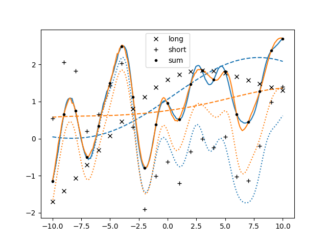
fig.savefig('components4.png')

If there was this more convenient way of dealing with latent components, why didn’t we introduce it right away? The reason is that it is not as general as managing the components manually with an explicit field. GP.addproc() defines processes which are independent of each other; to have nontrivial a priori correlations it is necessary to put the process index in the domain such that kernel can manipulate it. We did this at the end of Multidimensional output when we introduced an anticorrelation between the random walk components by multiplying the kernel with lgp.Categorical(dim='coord', cov=[[1, -0.99], [-0.99, 1]]).