4. Taking derivatives

The kernel of a derivative is the derivative of the kernel:

\[\begin{split}\operatorname{Cov}[f'(x), f'(x')] &= \frac \partial {\partial x} \frac \partial {\partial x'} \operatorname{Cov}[f(x), f(x')] = \\ &= \frac \partial {\partial x} \frac \partial {\partial x'} k(x, x').\end{split}\]

With lsqfitgp it’s easy to use derivatives of functions in fits (the automatic derivative calculations are implemented with jax). Let’s dive into the code:

import lsqfitgp as lgp
import numpy as np
import gvar

gp = lgp.GP(lgp.ExpQuad())
x = np.linspace(-5, 5, 200)
gp = (gp
    .addx(x, 'foo')
    .addx(x, 'bar', deriv=1)
)

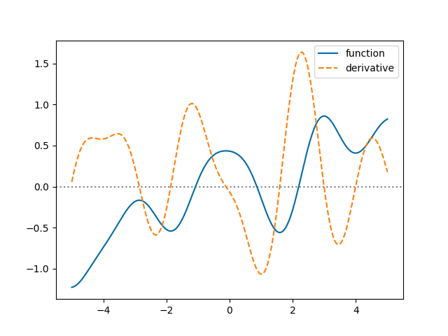
We said deriv=1 to addx(), easy as that. Let’s plot a sample from the prior:

from matplotlib import pyplot as plt

fig, ax = plt.subplots(num='lsqfitgp example')

y = gp.prior()
sample = gvar.sample(y)

ax.plot(x, sample['foo'], label='function')
ax.plot(x, sample['bar'], label='derivative', linestyle='--')
ax.axhline(0, linestyle=':', color='gray', zorder=-1)

ax.legend()

fig.savefig('derivatives1.png')

This time we used prior() without arguments, i.e., we did not specify if we wanted 'foo' or 'bar'. If you print sample, you will see it is a dictionary of arrays:

print(repr(sample))

Output:

BufferDict({
    'foo':
    array([-0.54830765, -0.44060242, -0.33276906, -0.22575309, -0.12042057,
            ...
            0.54683066,  0.51520693,  0.48205661,  0.44766003,  0.41235182]),
    'bar':
    array([ 2.13527672,  2.14804117,  2.14081828,  2.11552881,  2.07431084,
            ...
           -0.61230835, -0.64528377, -0.67311803, -0.69489595, -0.70976863]),
})

lsqfitgp (and also gvar) can work with arrays or dictionaries of arrays/scalars. This comes in handy to carry around all the numbers in one object without forgetting the names of things.

Looking at the plot, the points where the derivative is zero seem to correspond to minima/maxima of the function. Let’s check this more accurately:

condition = np.diff(np.sign(sample['bar'])) != 0
xcenter = 1/2 * (x[1:] + x[:-1])
zeros = xcenter[condition]

for zero in zeros:
    ax.axvline(zero, linestyle=':', color='gray', zorder=-1)

fig.savefig('derivatives2.png')

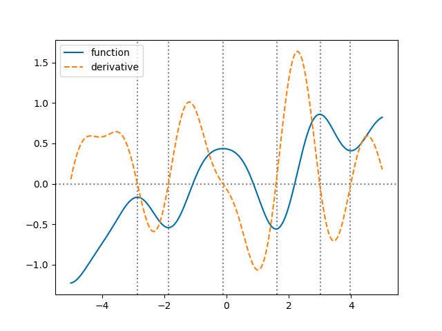
It works! Through the correlations, the prior “knows” that one line is the derivative of the other.

For a more realistic example, we add data. Imagine you have some datapoints, and that you also know that at a certain point the function has a maximum. You don’t know its value, but you know it must have a maximum. In terms of derivatives, a maximum is given by a zero first derivative and a negative second derivative. It won’t be complicated. I will stop using foo and bar and give meaningful names to the points:

x = np.array([-5, -4, -3, 3, 4, 5])
yerr = 0.1
y = np.cos(x) # we got bored of sines already
y += yerr * np.random.randn(len(x))
y = gvar.gvar(y, yerr * np.ones(len(x)))

gp = (lgp
    .GP(lgp.ExpQuad(scale=2))
    .addx(x, 'data')
    .addx(0, 'maximum-slope', deriv=1) # the cosine maximum is in 0
    .addx(0, 'maximum-curvature', deriv=2)
)

xplot = np.linspace(-6, 6, 200)
gp = gp.addx(xplot, 'plot')

given = {
    'data': y,
    'maximum-slope': 0, # exactly zero
    'maximum-curvature': gvar.gvar(-1, 0.3) # -1 ± 0.3
}

ypost = gp.predfromdata(given)

ax.cla()

ax.errorbar(x, gvar.mean(y), yerr=gvar.sdev(y), fmt='.k', capsize=2)
for sample in gvar.raniter(ypost, 4):
    deriv2 = sample['maximum-curvature']
    ax.plot(xplot, sample['plot'], label='deriv2 = {:.2f}'.format(deriv2))

ax.legend()

fig.savefig('derivatives3.png')

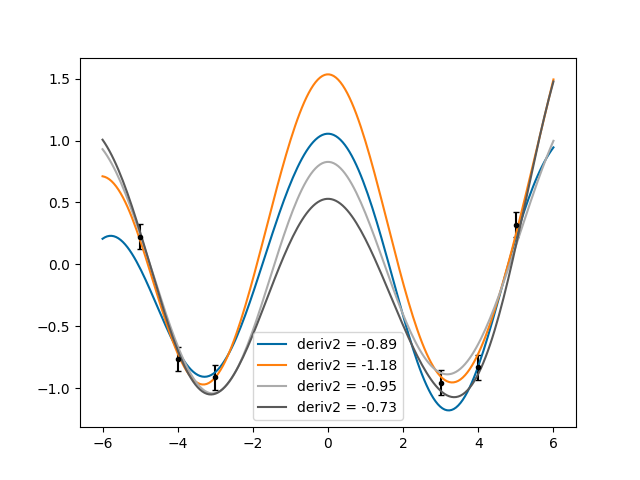
Very good! However, I’m cheating. I modified the scale parameter until I found that scale=2 would give something similar to a cosine. Try to guess what happens if you change the scale, and then try modifying it.