11. Hyperparameters
In the previous examples we often had to tweak the scale parameter of the
kernel to make it work. Whenever you’re tweaking a parameter, it would be nice
if the tweaking was done automatically. I would add: it would be nice to get
a statistical uncertainty on the optimal parameter value.
It is not possible to use what we have seen up to now to fit the scale
parameter, because that parameter goes into the definition of the kernel, and
the kernel completely specifies the Gaussian process. A different scale would
mean a different kernel and so a different Gaussian process.
This kind of parameters that reside on a “higher” level and can not be fitted
are called hyperparameters. In this context the “normal”, non-hyper parameters
are the values of the Gaussian process on the points you ask for them with
GP.predfromdata().
From a statistical point of view there’s no difference between parameters and hyperparameters, it is a practical categorization that comes up when the particular statistical tool you are using can not fit everything (our case), or because it’s something that you do not want to fit, or it is something that you want to call parameters but you already called parameters something else so you need another fancy name.
Enough chatter already, let’s fit this damn scale parameter:
import numpy as np
import lsqfitgp as lgp
import gvar

x = np.linspace(-5, 5, 11)
y = np.sin(x)
def makegp(hyperparams):
    return (lgp
        .GP(lgp.ExpQuad(scale=hyperparams['scale']))
        .addx(x, 'sine')
    )
hyperprior = {'log(scale)': gvar.log(gvar.gvar(3, 3))}
fit = lgp.empbayes_fit(hyperprior, makegp, {'sine': y}, raises=False)
print(fit.p['scale'])
Output:
2.16(17)
The code is short but introduces a bunch of new things, let’s go through it.
First, we encapsulated creating the GP object and adding points in
the function makegp, that takes as sole argument a dictionary of
hyperparameters.
Then we specified a “hyperprior” for the hyperparameters (if you want to fit
something you need a prior on it, there’s no way out of this). The function
makegp extracts a key 'scale' from the dictionary, but in the
hyperprior we used 'log(scale)'. This is a general feature of gvar,
that it can automatically apply the inverse of the transformation specified in
the key. It doesn’t work out of the box with any function: by default only the
logarithm is supported; you can add other functions with
gvar.BufferDict.add_distribution(), or use the copula module to define
them automatically.
This means that the parameter we are actually fitting is the logarithm of the
scale. Something like this is necessary because the scale must be a positive
number: if we put 'scale' in the hyperprior, the fitting routine would
explore negative values too, and we would get a loud error from Kernel.
Finally, we give everything to the class empbayes_fit: the hyperprior,
the gp-creating function, and a dictionary of data like we would pass to
predfromdata(). The attribute p is a dictionary containing the fit
result for the hyperparameters.
Now that we have found the optimal scale, we can use it to create a gp object and take some samples. However, since the hyperparameter has an uncertainty, we have to sample it too:
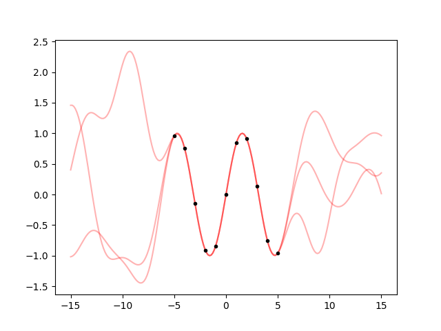
from matplotlib import pyplot as plt

fig, ax = plt.subplots(num='lsqfitgp example')

xplot = np.linspace(-15, 15, 200)

for hpsample in gvar.raniter(fit.p, 3):
    gp = makegp(hpsample).addx(xplot, 'plot')
    yplot = gp.predfromdata({'sine': y}, 'plot')

    for ysample in gvar.raniter(yplot, 1):
        ax.plot(xplot, ysample, color='red', alpha=0.3)

ax.plot(x, y, '.k')

fig.savefig('hyper1.png')
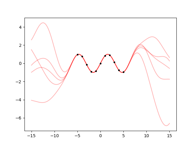
Cool. But I find the oscillations quite too high going away from the data. Can we change that with an hyperparameter? The amplitude of the oscillations is given by the prior variance, so we just need to multiply the kernel by a constant:
def makegp(hyperparams):
    kernel = hyperparams['sdev'] ** 2 * lgp.ExpQuad(scale=hyperparams['scale'])
    return (lgp
        .GP(kernel)
        .addx(x, 'sine')
    )

hyperprior = {
    'log(sdev)': gvar.log(gvar.gvar(1, 1)),
    'log(scale)': gvar.log(gvar.gvar(3, 3))
}

fit = lgp.empbayes_fit(hyperprior, makegp, {'sine': y}, raises=False)
print('sdev', fit.p['sdev'])
print('scale', fit.p['scale'])
Note
The function makegp must be jax-friendly. This means that operations that
involve hyperparameters must always be functional, i.e., you can not first
create an array and later assign values to it. Also, if you explicitly use
numpy functions, you have to do from jax import numpy instead of
import numpy. Read the jax documentation for detailed information.
Output:
sdev 2.44(81)
scale 2.86(22)
It did not do what I wanted! The fitted standard deviation is even higher than 1.
ax.cla()

for hpsample in gvar.raniter(fit.p, 5):
    gp = makegp(hpsample).addx(xplot, 'plot')
    yplot = gp.predfromdata({'sine': y}, 'plot')

    for ysample in gvar.raniter(yplot, 1):
        ax.plot(xplot, ysample, color='red', alpha=0.3)

ax.plot(x, y, '.k')

fig.savefig('hyper2.png')
I hate it when the fit does not give the right result. Ok, let’s calm down, math does not lie. If this is the result, and I think it’s wrong, then my assumptions are wrong. What are my assumptions? Well, I know it’s a sine, but I did’t tell this to the fit. I told it that the kernel is an exponential quadratic. The fit is trying to find a scale and variance such that it becomes as likely as possible to see a sine-like oscillation 10 units long with an exponential quadratic correlation.
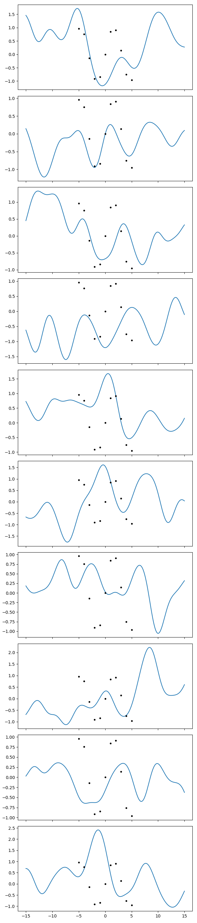
So we should deduce that such an oscillation typically comes out as a small oscillation in a more widely varying function. To get a feel of that, let’s plot a lot of samples from the prior with the hyperparameters I would have liked to come out, i.e., I’ll use a scale of 2 and a standard deviation of, say, 0.7:
gp = makegp({'scale': 2, 'sdev': 0.7}).addx(xplot, 'plot')

prior = gp.prior('plot')

fig.clf()
fig.set_size_inches(6.4, 30)
axs = fig.subplots(10, 1, sharex=True)

for ax, sample in zip(axs, gvar.raniter(prior)):
    ax.plot(xplot, sample)
    ax.plot(x, y, '.k')

fig.tight_layout()
fig.savefig('hyper3.png')
Now we do the same with the optimized hyperparameters:
gp = makegp(fit.pmean).addx(xplot, 'plot')

prior = gp.prior('plot')

for ax, sample in zip(axs, gvar.raniter(prior)):
    ax.cla()
    ax.plot(xplot, sample)
    ax.plot(x, y, '.k')

fig.savefig('hyper4.png')
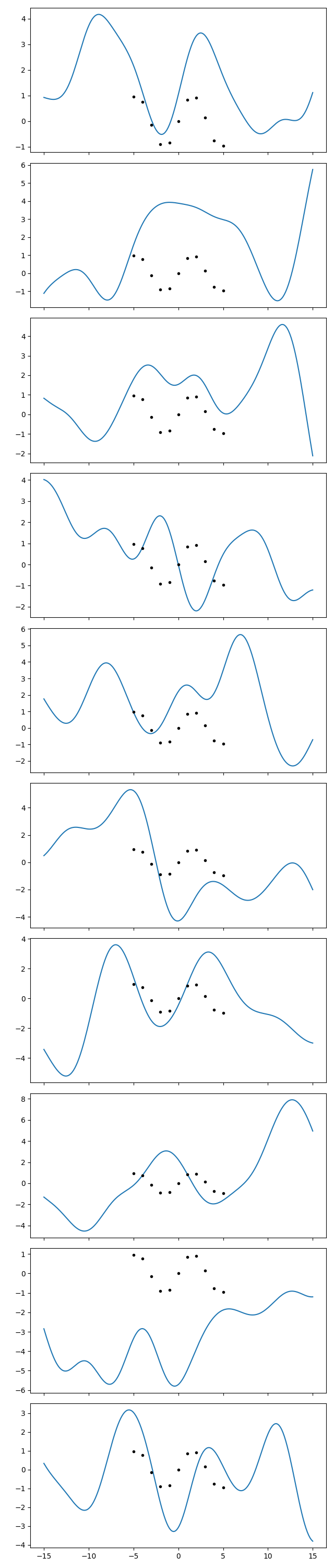
In the first series of plots I see 2-3 curves that do something similar to the
datapoints. I can find 2-3 in the second series too. So ok, I acknowledge that
those points can likely come out even with a wider variance than I thought.
But I recall the fit saying sdev 2.44(81). This is \(2.4 \pm 0.8\), so
the uncertainty is a bit wide, but still 1 seems far from the mean. What
probability is the fit giving to sdev being less than 1? We can compute this by
integrating the Gaussian distribution, with the caveat that the parameter we
actually used in the fit is log(sdev):
from scipy import stats

p = fit.p['log(sdev)']
prob = stats.norm.cdf(np.log(1), loc=gvar.mean(p), scale=gvar.sdev(p))
print('{:.3g}'.format(prob))
Output:
0.00383
Ouch, that’s low. The fit values my intuition at less than 1 %. Now I’m
outraged, I’ll show lsqfitgp that he’s wrong and I’m right. I’ll do a
proper bayesian fit with Markov Chains using pymc3. First, I print
the mean and standard deviations of the effective hyperparameters (the
logarithms):
for k, v in fit.p.items():
    print(k, v)
Output:
log(sdev) 0.89(33)
log(scale) 1.051(77)
Then I run this code to get the (I hope) correct and satisfying answer:
import pymc3 as pm

model = pm.Model()
with model:
    logscale = pm.Normal('logscale', mu=np.log(3), sigma=1)
    logsdev = pm.Normal('logsdev', mu=np.log(1), sigma=1)
    kernel = pm.math.exp(logsdev) ** 2 * pm.gp.cov.ExpQuad(1, ls=pm.math.exp(logscale))
    gp = pm.gp.Marginal(cov_func=kernel)
    gp.marginal_likelihood('data', x[:, None], y, 0)

with model:
    mp = pm.find_MAP()
    trace = pm.sample(10000, cores=1)

print('\nMaximum a posteriori (must be the same as lsqfitgp):')
print('log(sdev) {:.2f}'.format(mp['logsdev']))
print('log(scale) {:.2f}'.format(mp['logscale']))

df = pm.trace_to_dataframe(trace)
mean = df.mean()
cov = df.cov()

meandict = {}
covdict = {}
for label1 in df.columns:
    meandict[label1] = mean[label1]
    for label2 in df.columns:
        covdict[label1, label2] = cov[label1][label2]

params = gvar.gvar(meandict, covdict)
print('\nPosterior mean and standard deviation:')
print('log(sdev)', params['logsdev'])
print('log(scale)', params['logscale'])

p = params['logsdev']
prob_gauss = stats.norm.cdf(np.log(1), loc=gvar.mean(p), scale=gvar.sdev(p))
true_prob = np.sum(df['logsdev'] <= np.log(1)) / len(df)
print('\nProbability of having sdev < 1:')
print('prob_gauss {:.3g}'.format(prob_gauss))
print('true_prob {:.3g}'.format(true_prob))
Output:
logp = -108.32, ||grad|| = 2,021.1: 100%|█████████████████████████████████████████████████████████████████| 20/20 [00:00<00:00, 228.23it/s]
Auto-assigning NUTS sampler...
Initializing NUTS using jitter+adapt_diag...
Sequential sampling (2 chains in 1 job)
NUTS: [logsdev, logscale]
Sampling chain 0, 0 divergences: 100%|███████████████████████████████████████████████████████████████| 10500/10500 [03:41<00:00, 47.38it/s]
Sampling chain 1, 0 divergences: 100%|███████████████████████████████████████████████████████████████| 10500/10500 [03:37<00:00, 48.17it/s]
The number of effective samples is smaller than 25% for some parameters.

Maximum a posteriori (must be the same as lsqfitgp):
log(sdev) 0.89
log(scale) 1.05

Posterior mean and standard deviation:
log(sdev) 0.86(40)
log(scale) 1.01(11)

Probability of having sdev < 1:
prob_gauss 0.0151
true_prob 0.0165
So the correct mean and standard deviation for log(sdev) are \(0.86 \pm
0.40\), versus lsqfitgp’s result \(0.89 \pm 0.33\). The probability
of having sdev < 1 is 1.5 %, and by doing a more accurate computation that
keeps into account that the distribution is actually non-Gaussian I manage to
get it to 1.6 %, four times as much as lsqfitgp’s answer, but still low.
What did we learn? First, that empbayes_fit is not so accurate, it
just gives a reasonable estimate of the mean and covariance matrix of the
posterior for the hyperparameters. This is because it is much faster than, for
example, pymc3 (tipically just starting up pymc3 takes more time
than doing a fit with lsqfitgp). So, when computing sensitive quantities
like the probability of a tail of the distribution, the result can become quite
wrong.
Second, we learned that I was wrong and effectively it is not very likely, with the exponential quadratic kernel, to get an harmonic oscillation with a prior variance less than 1.
Is there a somewhat clear explanation of this? In More on kernels, we said that any kernel can be written as
What are the \(h_i\) for the exponential quadratic kernel? Well, first I have to say that I’ll actually do an integral instead of a summation, but whatever. The solution is, guess what, Gaussians:
This means that the fit is trying to redraw the datapoints using a combination of Gaussians, so it will be happy when the datapoints are similar to a bunch of Gaussians, such that it doesn’t have to figure out a nontrivial mixture of many different Gaussians that magically gives out precisely our points.
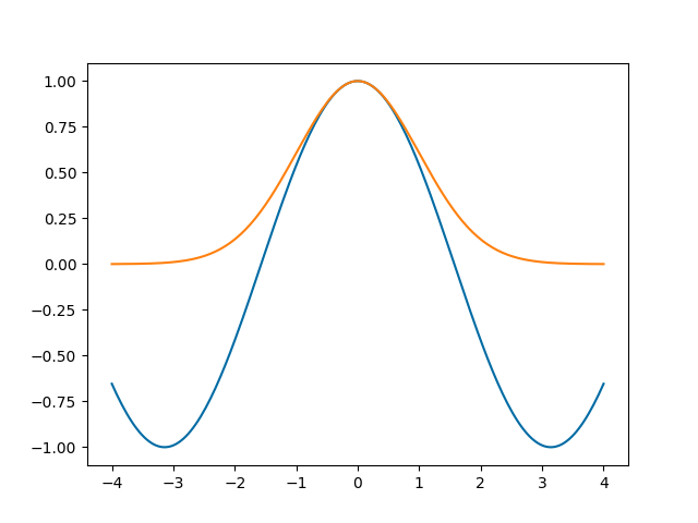
But isn’t a sine similar to some Gaussians, one up, one down, etc.? Apparently so. Let’s explore this impression by plotting a sine aligned with a Gaussian. To align them, I will put the maxima in the same point, and also make them have the same second derivative:
x = np.linspace(-4, 4, 200)
cos = np.cos(x)
gauss = np.exp(-1/2 * x**2)

fig, ax = plt.subplots(num='cosgauss')

ax.plot(x, cos)
ax.plot(x, gauss)

fig.savefig('hyper5.png')
Ok. Can we get a better alignment? The fit wanted the Gaussian to be higher than the sine, so let’s try it:
gauss_large = 3 * np.exp(-1/2 * (x / np.sqrt(3)) ** 2) - 2
ax.plot(x, gauss_large, scaley=False)

fig.savefig('hyper6.png')
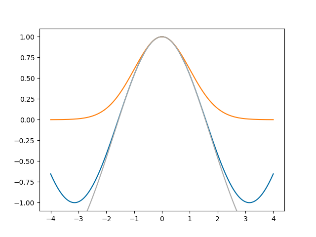
So the fit sees that a sine is more similar to the top of a high Gaussian than to a Gaussian with the same height as the sine.
We learned a lesson. But now how do we make the fit work? Oh well that’s as
easy as cheating actually if we use the Periodic kernel:
x = np.linspace(-5, 5, 11)

def makegp(hp):
    scale = hp['period'] / (2 * np.pi)
    kernel = lgp.Periodic(scale=scale)
    return (lgp
        .GP(kernel)
        .addx(x, 'sine')
    )

hprior = {
    'log(period)': gvar.log(2 * np.pi * gvar.gvar(1, 1)),
}
fit = lgp.empbayes_fit(hprior, makegp, {'sine': y}, raises=False)
for k in fit.p.all_keys():
    print(k, fit.p[k])

ax.cla()

for hpsamp in gvar.raniter(fit.p, 3):
    gp = makegp(hpsamp).addx(xplot, 'plot')
    yplot = gp.predfromdata({'sine': y}, 'plot')

    for ysamp in gvar.raniter(yplot, 1):
        ax.plot(xplot, ysamp, alpha=0.3)
    ax.plot(x, y, '.k')

fig.savefig('hyper7.png')
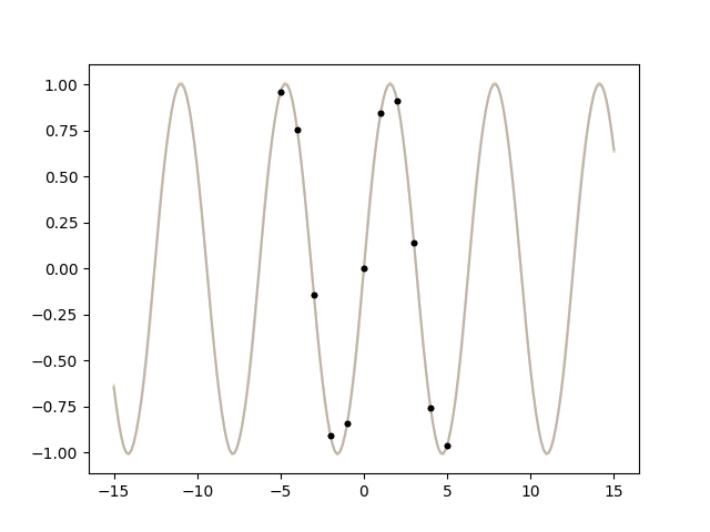
Output:
log(period) 1.8373(29)
period 6.280(18)