10. Splitting components
In More on kernels we saw an example where we summed two ExpQuad
kernels with different scale, and the result effectively looked like the sum
of two processes, because the kernel of a sum of processes is the sum of their
kernels.
When summing processes it is useful to get the fit result separately for each component. We first generate some data:
import numpy as np
import lsqfitgp as lgp
import gvar
from matplotlib import pyplot as plt

kernel_long = 10 * lgp.ExpQuad(scale=10)
kernel_short = lgp.ExpQuad(scale=1)

x = np.linspace(-10, 10, 21)
fakedata = {}
fakedata['long'] = gvar.sample(lgp.GP(kernel_long).addx(x, 'A').prior('A'))
fakedata['short'] = gvar.sample(lgp.GP(kernel_short).addx(x, 'A').prior('A'))
fakedata['sum'] = fakedata['long'] + fakedata['short']

fig, ax = plt.subplots(num='lsqfitgp example')

ax.plot(x, fakedata['sum'], '.k')

fig.savefig('components1.png')
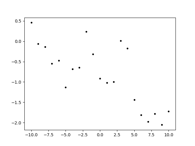
We defined two processes with different correlation lengths, sampled from each, and summed the result to make our fake data. Generating fake data from the prior is a good way to test a statistical procedure.
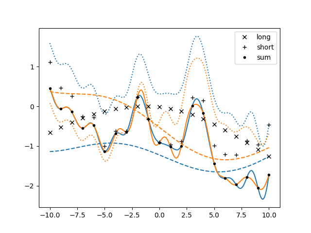
We also saved the data generated for each component. Our goal is to recover the
components by using only the sum. We start by creating a GP object without
specifying a kernel:
gp = lgp.GP()
Then we add separately the two kernels to the object using GP.defproc:
gp = (gp
    .defproc('long', kernel_long)
    .defproc('short', kernel_short)
)
Now the two names 'long' and 'short' stand for a priori independent
processes with their respective kernels. These names reside in a namespace
separate from the one used by addx, addlintransf, etc. Now we
use these to define the sum as a process:
gp = gp.deflintransf('sum',
    lambda l, s: lambda x: l(x) + s(x),
    ['long', 'short'])
The method deflintransf is analogous to addlintransf but works
for a whole process at once. What we are doing mathematically is the
following:
The second argument to the method is a function that takes in two functions, and outputs a new function. The third argument specifies which processes are to be transformed in such way.
Now that we have defined all the processes we care about, we evaluate them on the points:
xplot = np.linspace(-10, 10, 200)

gp = (gp
    .addx(x, 'datalong' , proc='long' )
    .addx(x, 'datashort', proc='short')
    .addx(x, 'datasum'  , proc='sum'  )

    .addx(xplot, 'plotlong' , proc='long' )
    .addx(xplot, 'plotshort', proc='short')
    .addx(xplot, 'plotsum'  , proc='sum'  )
)
We specified the processes using the proc parameter of addx. Then we
continue as usual:
post = gp.predfromdata({
    'datasum': fakedata['sum'],
}, ['plotlong', 'plotshort', 'plotsum'])

ax.cla()

for sample in gvar.raniter(post, 2):
    line, = ax.plot(xplot, sample['plotsum'])
    color = line.get_color()
    ax.plot(xplot, sample['plotlong'], '--', color=color)
    ax.plot(xplot, sample['plotshort'], ':', color=color)

for marker, key in zip(['x', '+', '.'], ['long', 'short', 'sum']):
    ax.plot(x, fakedata[key], color='black', marker=marker, label=key, linestyle='')
ax.legend()

fig.savefig('components4.png')
GP.defproc can only define a priori independent processes. To have a priori
correlations it would be necessary to define a single process over an extended
input, with an explicit index indicating the component, such that the kernel can
act on it. We did this at the end of Multidimensional output when we introduced an
anticorrelation between the random walk components by multiplying the kernel
with lgp.Categorical(dim='coord', cov=[[1, -0.99], [-0.99, 1]]).