5. Taking integrals
There is no “direct” support for integrals in lsqfitgp. There’s not
something like a deriv=-1 option for GP.addx(). However, since the
data can be specified for the derivative of the process, it is possible to do
integrals by defining the process for the integral and then fitting its
derivative.
Let’s compute the primitive of our dear friend cosine:
import lsqfitgp as lgp
import numpy as np
import gvar

x = np.linspace(-5, 5, 11)
y = np.cos(x)
xplot = np.linspace(-5, 5, 200)

gp = (lgp
    .GP(lgp.ExpQuad(scale=2))
    .addx(xplot, 'primitive')
    .addx(x, 'cosine', deriv=1)
)

yplot = gp.predfromdata({'cosine': y}, 'primitive')
We gave the data for the 'cosine' label which has deriv=1, and asked for
the posterior on the label 'primitive' which is not derived. Now we plot:
from matplotlib import pyplot as plt

fig, ax = plt.subplots(num='lsqfitgp example')

ax.plot(x, y, '.k')
for sample in gvar.raniter(yplot, 8):
    ax.plot(xplot, sample, color='blue', alpha=0.5, zorder=-1)

fig.savefig('integrals1.png')
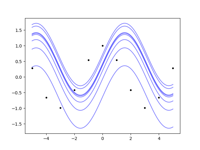
So, the Gaussian process not only can do integrals, it also understands that the primitive is defined up to an additive constant.
How can we do a definite integral? There’s the easy way, and the easy but not
obvious way. Let’s go first with the easy one: we use the correlation tracking
features of gvar.
area = yplot[-1] - yplot[0] # -1 means the last index
print(area)
Output: -1.9157(27). The (27) is a short notation for saying that the
standard deviation is 0.0027. Is it correct? Well we know the answer here:
true_area = np.sin(xplot[-1]) - np.sin(xplot[0])
print(true_area, area - true_area)
Output: -1.917848549326277 0.0022(27). So it’s correct within one standard
deviation.
The not obvious way follows:
gp = gp.addlintransf(lambda x: x[-1] - x[0], ['primitive'], 'integral')
area = gp.predfromdata({'cosine': y}, 'integral')
print(area)
Output: -1.9157(27). What did we do? addlintransf() is similar to
addx(), but instead of adding new points where the process is
evaluated, it defines a linear transformation of already specified process
values. The first argument is lambda x: x[-1] - x[0], a function which
takes in an array and computes the same difference we computed by hand before.
The second argument is ['primitive'], a list of labels that indicate which
arrays are passed to the function. The last argument is the name of the newly
defined array of process values, as in addx().
Using addlintransf() for this is overkill, since transformations
applied to the posterior can always be applied directly to the arrays returned
by predfromdata(). It becomes useful when there’s data to fit against
the transformed quantities.
Example: you already know the area of the function. Let’s try this with a Cauchy pdf, pretending we only know its area and some values of the function not too close to the center:
from scipy import stats

x = np.array([-5, -4, -3, -2, 2, 3, 4, 5])
xplot = np.linspace(-5, 5, 200)

true_function = stats.cauchy.pdf
true_area = np.subtract(*stats.cauchy.cdf([x[-1], x[0]]))

y = true_function(x)

gp = (lgp
    .GP(lgp.ExpQuad(scale=2))
    .addx(x, 'datapoints', deriv=1)
    .addx(xplot, 'plot', deriv=1)
    .addx(-5, 'left')
    .addx(5, 'right')
    .addlintransf(lambda l, r: r - l, ['left', 'right'], 'area')
)

yplot = gp.predfromdata({'datapoints': y, 'area': true_area}, 'plot')

ax.cla()

m = gvar.mean(yplot)
s = gvar.sdev(yplot)
ax.fill_between(xplot, m - s, m + s, alpha=0.5)
ax.plot(xplot, true_function(xplot), color='gray', linestyle='--')
ax.plot(x, y, '.k')

fig.savefig('integrals2.png')
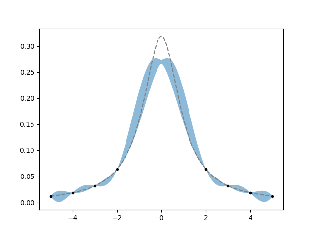
It doesn’t work too well, the posterior band completely misses the top of the function, but at least it gets the sides right. This highlights the importance of the choice of prior. Try playing with changing the kernel and its parameters too see if you can find a prior that “likes” the Cauchy pdf enough to reproduce it given the constraints.