3. More on kernels
In First example: a sine, we defined the kernel as the function that gives the covariance of the process values at two different points:
So you can imagine the Gaussian process as a multivariate Gaussian distribution on an infinitely long vector \(f(x)\), where \(x\) is a “continuous index”, and \(k(x, x')\) is the covariance matrix.
This implies that kernels are symmetric, i.e., \(k(x, x') = k(x', x)\). Also, covariance matrices must be positive semidefinite (explanation on wikipedia). For kernels, this means that, for any function \(g\),
This is the reason why you can’t pick any two-variable symmetric function as kernel. So, how do you build valid kernels? Luckily, there are some simple rules that allow to make kernels out of other kernels:
The sum of kernels is a kernel.
The product of kernels is a kernel.
Corollary 1: a kernel can be multiplied by a nonnegative constant.
Corollary 2: a kernel can be raised to an integer power (some kernels allow non-integer nonnegative powers, they are called “infinitely divisible”).
Corollary 3: a function with nonnegative Taylor coefficients applied to some kernels is a valid kernel.
Now we need a set of fundamental kernels to start with. There is a class of functions that can be easily shown to be positive semidefinite (exercise for the reader): \(k(x, x') = h(x) h(x')\) for some function \(h\). In fact, it can be shown that any kernel can be written as
for some possibly infinite set of functions \(\{h_i\mid i=0,1,\ldots\}\).
Ok, but if I use a kernel of the form \(h(x) h(x')\), how will it behave in practice with the data?
Let’s suppose that you have some data \(y(x)\) that you want to fit with a specific function, that (let’s say by chance) we call \(h(x)\), apart from an amplitude parameter, i.e., the model is
where \(\varepsilon(x)\) is an independent zero mean Gaussian distributed error. Put a Gaussian prior with zero mean and unit variance on the parameter \(p\). What is the prior covariance of \(y(x)\) with \(y(x')\)? Let’s compute:
This, by definition, is also the prior of a Gaussian process fit with kernel \(h(x) h(x')\). It can be extended to \(y = \sum_i p_i h_i(x)\) to get the general kernel from above (exercise). So, have we discovered that a Gaussian process fit is just a linear least squares fit with priors? Yes! But, when thinking in terms of Gaussian processes, you normally use an infinite set of functions \(h_i\). You don’t even think about it in terms of the \(h_i\), because the kernel has meaning in itself.
Let’s now build some feeling for how kernels behave. In First example: a sine we always
used the ExpQuad kernel. To start, we will sum two exponential
quadratic kernels with different scales, and see what happens:
import lsqfitgp as lgp
import numpy as np
import gvar
from matplotlib import pyplot as plt

kernel = lgp.ExpQuad(scale=0.3)
kernel += 3**2 * lgp.ExpQuad(scale=10) # we also multiply the scale=10
                                       # kernel to see it better
gp = lgp.GP(kernel)

x = np.linspace(-15, 15, 300)
gp = gp.addx(x, 'baz')

fig, ax = plt.subplots(num='lsqfitgp example')

y = gp.prior('baz')
for sample in gvar.raniter(y, 1):
    ax.plot(x, sample)

fig.savefig('kernels1.png')
First thing to notice, we introduced another GP method:
prior(). It returns an array of GVar variables representing
the prior. In general it is useful to plot some samples from the prior to
understand if the kernel makes sense before putting the data in.
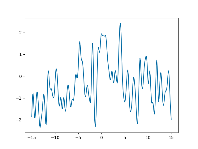
Looking at the plot, we see the function oscillates rapidly, but the center of the oscillation drifts. Effectively, if you think about it, summing two kernels is like summing two independent Gaussian processes: let \(f_1\) and \(f_2\) be processes with kernels \(k_1\) and \(k_2\) respectively, then the kernel of \(f_1 + f_2\) is
So we are looking at the sum of two processes, one ExpQuad(scale=0.3)
and one ExpQuad(scale=10).
Let’s now multiply kernels. The \(h(x)h(x')\) kernel is implemented in
lsqfitgp as Rescaling. We multiply it by an exponential
quadratic:
lorentz = lambda x: 1 / (1 + x**2)
kernel = lgp.ExpQuad() * lgp.Rescaling(stdfun=lorentz)
gp = (lgp
    .GP(kernel)
    .addx(x, 'baz')
)

ax.cla()

y = gp.prior('baz')
sample = next(gvar.raniter(y, 1))
ax.plot(x, sample)

fig.savefig('kernels2.png')
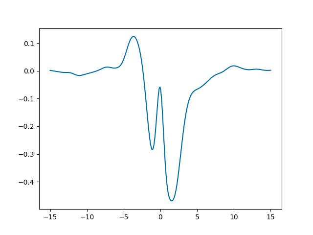
The function oscillates, but the oscillations are suppressed going away from
zero. This is because the function we defined, lorentz, goes to zero for
\(x\to\pm\infty\). Let’s plot a band delimited by \(\pm\) that
function (cyan), and the band of the standard deviation of y (yellow):
ax.fill_between(x, -lorentz(x), lorentz(x), color='cyan', alpha=0.5)
ax.fill_between(x, -gvar.sdev(y), gvar.sdev(y), color='yellow', alpha=0.5)

fig.savefig('kernels3.png')
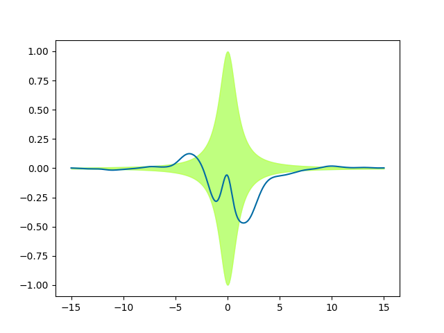
We see only one green (cyan+yellow) band, because it is a perfect match. We
have rescaled the standard deviations of the prior with the function
lorentz, without changing the correlations. Since the ExpQuad
prior variance is 1 everywhere, after the multiplication it just matches
lorentz(x).