13. Nonlinear models
Using GP we can define a Gaussian process. Using GP.addlintransf we can
represent finite linear transformations of the process, and we can take
derivatives with GP.addx. This means that we can only do linear operations on
the process before putting the data in.
A common non-linear operation is putting a boundary on the possible data values. Gaussian distributions don’t play nicely with boundaries—they are defined on \((-\infty,\infty)\)—so it is necessary to map the Gaussian process space to an interval with a nonlinear function.
lsqfitgp is designed to work with the general purpose fitting module
lsqfit (after which it takes the name) for this kind of situations. If
you want to know more, it has a good documentation.
Let’s see how to fit some data that is constrained in (-1, 1). To map the Gaussian process space to the data space, we’ll use a hyperbolic tangent. It has the properties \(\tanh(\pm\infty) = \pm 1\), \(\tanh'(0) = 1\), \(\tanh(-x) = -\tanh(x)\).
We first define a Gaussian process as usual and take a sample from it as fake data.
import lsqfitgp as lgp
import numpy as np
import gvar

gp = lgp.GP(lgp.ExpQuad())

x = np.arange(15)
gp = gp.addx(x, 'data')

data_gp = gvar.sample(gp.prior('data'))
Then we map it to (-1, 1):
data = np.tanh(data_gp)
Note that we first sampled the latent Gaussian process obtaining data_gp,
and then passed it through our nonlinear function to obtain the fake data. A
possibly serious mistake would be to do the converse, first passing the prior
through the nonlinear function, with np.tanh(gp.prior('data')), and then
sampling from it. To see this intuitively, consider that in the latter case the
fake data would not satisfy the requirement of being bounded within (-1, 1).
Now we’ll add errors to the data. If data does not have errors, there’s not
really a problem to start with: you can map the data to \((-\infty,
\infty)\) with arctanh, do the Gaussian process fit, take some
samples, map the samples back with tanh.
You may do that even with errors, either at first order using
gvar.arctanh, or by transforming the errors manually yourself. However,
in that way you would be doing a fit with Gaussian errors on the transformed
data. What we will do is a fit with Gaussian errors on the data itself. Another
case we won’t explore in which just transforming the data before the fit is not
sufficient is when the mapping between the Gaussian process and the data
depends on a fit parameter.
err = 0.1
rng = np.random.default_rng([2023, 8, 23, 17, 18])
data += err * rng.standard_normal(len(data))
data = gvar.gvar(data, np.full_like(data, err))
Then as usual we add a finer grid of points where we will compute the prediction:
xplot = np.linspace(-10, 25, 200)
gp = gp.addx(xplot, 'plot')
Now we define the prior and model function following the requirements of
lsqfit.nonlinear_fit and run the fit:
import lsqfit

prior = {
    'gproc': gp.prior('data')
}

def fcn(params):
    return gvar.tanh(params['gproc'])

fit = lsqfit.nonlinear_fit(data=data, fcn=fcn, prior=prior)
print(fit.format(maxline=True))
Output:
Least Square Fit:
  chi2/dof [dof] = 1.1 [15]    Q = 0.36    logGBF = -11.047

Parameters:
        gproc 0   -0.15 (10)     [  0.0 (1.0) ]
              1    0.71 (15)     [  0.0 (1.0) ]
              2   -1.30 (34)     [  0.0 (1.0) ]  *
              3   -2.37 (56)     [  0.0 (1.0) ]  **
              4   -1.20 (30)     [  0.0 (1.0) ]  *
              5    0.58 (13)     [  0.0 (1.0) ]
              6    0.55 (13)     [  0.0 (1.0) ]
              7    0.24 (10)     [  0.0 (1.0) ]
              8   -0.52 (12)     [  0.0 (1.0) ]
              9   -0.41 (11)     [  0.0 (1.0) ]
             10    0.54 (13)     [  0.0 (1.0) ]
             11    0.86 (18)     [  0.0 (1.0) ]
             12    0.51 (12)     [  0.0 (1.0) ]
             13    0.33 (11)     [  0.0 (1.0) ]
             14    0.15 (10)     [  0.0 (1.0) ]

Fit:
      key        y[key]      f(p)[key]
--------------------------------------
        0    -0.17 (10)    -0.149 (99)
        1     0.67 (10)     0.610 (97)
        2    -0.99 (10)    -0.861 (88)  *
        3    -0.91 (10)    -0.983 (19)
        4    -0.92 (10)    -0.832 (91)
        5     0.57 (10)     0.523 (97)
        6     0.47 (10)     0.500 (96)
        7     0.26 (10)     0.235 (98)
        8    -0.50 (10)    -0.476 (96)
        9    -0.39 (10)    -0.388 (97)
       10     0.50 (10)     0.494 (96)
       11     0.71 (10)     0.696 (93)
       12     0.46 (10)     0.467 (97)
       13     0.33 (10)     0.322 (98)
       14     0.15 (10)     0.152 (99)

Settings:
  svdcut/n = 1e-12/0    tol = (1e-08,1e-10,1e-10*)    (itns/time = 22/0.1)
  fitter = scipy_least_squares    method = trf
Let’s plot everything. First we compute the posterior on the xplot points:
gpplot = gp.predfromfit({'data': fit.p['gproc']}, 'plot')
This time we use GP.predfromfit instead of the usual
GP.predfromdata. This method takes into account that the distribution
represented by fit.p['gproc'] is not the uncertainty of some datapoints,
but is already the distribution of some points of our process. We want to
“extend” fit.p['gproc'], not condition on it.
Then we inject the extended posterior into a copy of the fit result dictionary:
fitp = dict(fit.p)     # dict() makes a copy of fit.p
fitp['gproc'] = gpplot
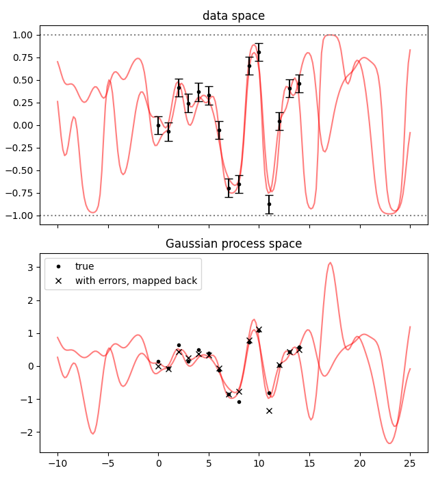
This copy-and-replace step is a bit redundant here, it is for when there are also other parameters beside the Gaussian process, and we do not want to modify the fit result dictionary for good bookkeeping practice. Then we plot both the data space and the Gaussian process space.
from matplotlib import pyplot as plt

fig, axs = plt.subplots(2, 1, sharex=True, num='lsqfitgp example', figsize=[6.4, 7])

for sample in gvar.raniter(fitp, 2):
    axs[0].plot(xplot, fcn(sample), color='red', alpha=0.5)
    axs[1].plot(xplot, sample['gproc'], color='red', alpha=0.5)

ax = axs[0]
ax.set_title('data space')
for boundary in 1, -1:
    ax.axhline(boundary, color='gray', linestyle=':')
ax.errorbar(x, gvar.mean(data), yerr=gvar.sdev(data), fmt='.k', capsize=4)

ax = axs[1]
ax.set_title('Gaussian process space')
ax.plot(x, data_gp, '.k', label='true')
ax.plot(x, np.arctanh(gvar.mean(data)), 'xk', label='with errors, mapped back')
ax.legend()

fig.tight_layout()
fig.savefig('nonlinear1.png')