7. Multidimensional input

lsqfitgp supports multidimensional input through numpy structured arrays. Elements of structured arrays have named fields:

import numpy as np

x = np.linspace(-3, 3, 30)
y = np.linspace(-3, 3, 30)

xy = np.empty((len(x), len(y)), dtype=[('x', float), ('y', float)])
xy['x'] = x[:, None]
xy['y'] = y[None, :]

Here we used a bit of Numpy indexing and broadcasting to fill a 30x30 array xy with a grid of x, y coordinates. We specified a data type [('x', float), ('y', float)] for the array xy, this means that each element of xy is a pair of numbers. We specified a shape (len(x), len(y)), where x and y are the two linspaces, and then filled separately the 'x' and 'y' fields of the xy elements with the linspaces. xy is a 2D array, while x and y are 1D, so using None we added a dummy dimension along which the copying is repeated. The colons : are empty slices and leave the dimension untouched.

It is not important for xy to be a 2D array because we are using bidimensional points, it is just a convenience for building a rectangular grid. Do not confuse the number of dimensions of the array with the number of fields in its elements.

We only used 30 points for the side of the grid. This is because 30x30 = 900 and at around 1000 datapoints lsqfitgp starts being slow. This is an inherent limitation of Gaussian processes, which can be overcome only with approximations or specialized algorithms.

Now we put xy into a GP as usual and extract a sample from the prior.

import lsqfitgp as lgp
import gvar

gp = (lgp
    .GP(lgp.ExpQuad())
    .addx(xy, 'foo')
)

prior = gp.prior('foo')
sample = gvar.sample(prior)

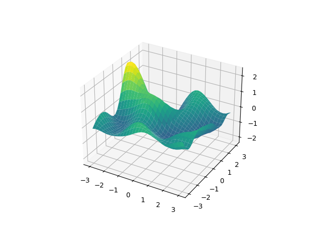
We plot the sample in 3d:

from matplotlib import pyplot as plt

fig, ax = plt.subplots(num='lsqfitgp example', subplot_kw=dict(projection='3d'))

ax.plot_surface(xy['x'], xy['y'], sample, cmap='viridis')

fig.savefig('in1.png')

We got a nice random surface. The ExpQuad kernel just worked out of the box with multidimensional input. What kernel are we using really? ExpQuad is a subclass of IsotropicKernel. This means it only depends on the distance between points, i.e., it doesn’t care what the input is as long as it can apply Pythagoras’ theorem. So the kernel we used is:

\[k(x_1, y_1, x_2, y_2) = \exp \left( -\frac {(x_1 - x_2)^2 + (y_1 - y_2)^2} 2 \right).\]

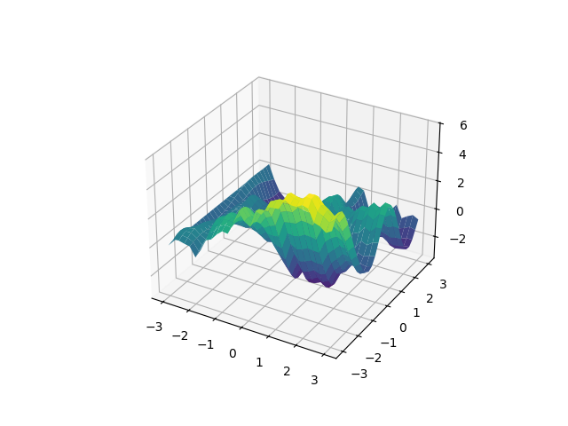
We can do more sophisticated things if we control how the kernel acts on each dimension. Let’s use a random walk along \(x\) and an exponential quadratic along \(y\):

gp = (lgp
    .GP(lgp.Wiener(dim='x', loc=-3) * lgp.ExpQuad(dim='y'))
    .addx(xy, 'foo')
)

prior = gp.prior('foo')
sample = gvar.sample(prior)

ax.cla()
ax.plot_surface(xy['x'], xy['y'], sample, cmap='viridis')

fig.savefig('in2.png')

Uhm, quite unelegant. I don’t like random walks any more. We used the dim keyword to specify the dimension, and loc=-3 to translate the random walk (it raises an error if it gets negative input points).

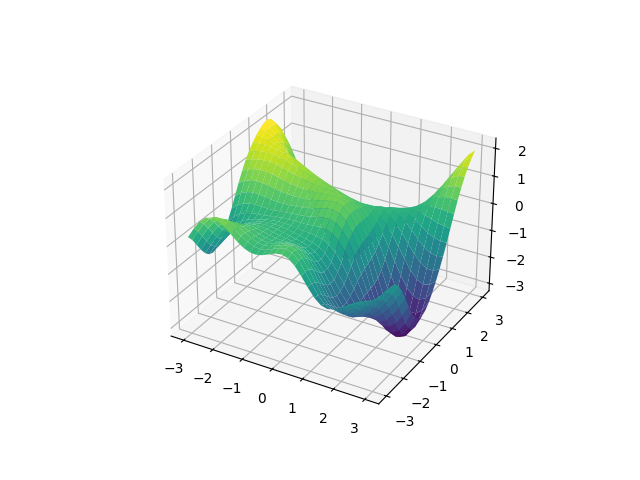
In many dimensions it can get tedious to specify all the field names, it would be simpler if multidimensional input was implemented with arrays. Luckily numpy supports array data types in fields. Let’s redo the first example, this time without named fields:

xy = np.empty((len(x), len(y)), dtype=[('foo', float, 2)])
xy['foo'][..., 0] = x[:, None]
xy['foo'][..., 1] = y[None, :]

Ok, I lied a bit, there’s still a field name around. It is needed because otherwise lsqfitgp would not know that the last axis with size 2 is a 2-dimensional point instead of a pair of points, so we encapsulate it in a field. numpy treats the ellipsis ... as a string of colons : of the appropriate length.

gp = (lgp
    .GP(lgp.ExpQuad())
    .addx(xy, 'foo')
)

prior = gp.prior('foo')
sample = gvar.sample(prior)

ax.cla()
ax.plot_surface(xy['foo'][..., 0], xy['foo'][..., 1], sample, cmap='viridis')

fig.savefig('in3.png')

However, with this method, it is not possible to apply a kernel only along a specific dimension. A kernel can be applied only on everything or on a single whole named field. By splitting your dimensions in named fields with different shapes this should still be flexible enough. To do arbitrary manipulations, write your own kernel.