9. Multidimensional output

lsqfitgp has no “direct” support for multidimensional output. However, as the derivative functionality can be used to take integrals, multidimensional input can be used to implement multidimensional output.

Let \(f:X \to \mathbb R^n\). Consider the components of the function \(f_i(x), i = 1,\ldots,n\). Formally we can also write this as \(f(i, x)\), so an n-dimensional function is like a one-dimensional function with an additional integer input dimension.

Let’s try to implement a random walk on a plane. A random walk is the sum of small independent increments. A random step on a plane is an increment along x and one along y, so it is equivalent to two 1D random walks stacked into a vector.

import numpy as np

time = np.linspace(0, 0.1, 300)
x = np.empty((2, len(time)), dtype=[('time', float), ('coord', int)])
x['time'] = time[None, :]
x['coord'] = np.arange(2)[:, None]

We have created a 2D input array with a dimension for time and another for the output coordinate indicator. The array is a grid where the first axis coordinate corresponds to the output coordinate.

import lsqfitgp as lgp

gp = (lgp
    .GP(lgp.Wiener(dim='time') * lgp.White(dim='coord'))
    .addx(x, 'walk')
)

We use a Wiener kernel (a random walk) on the 'time' field multiplied with a White kernel (white noise, no correlations) on the 'coord' field.

Just for fun, we’ll force the random walk to arrive at the (1, 1) point:

import gvar
from matplotlib import pyplot as plt

end = np.empty(2, dtype=x.dtype)
end['time'] = np.max(time)
end['coord'] = np.arange(2)
gp = gp.addx(end, 'endpoint')

path = gp.predfromdata({'endpoint': [1, 1]}, 'walk')

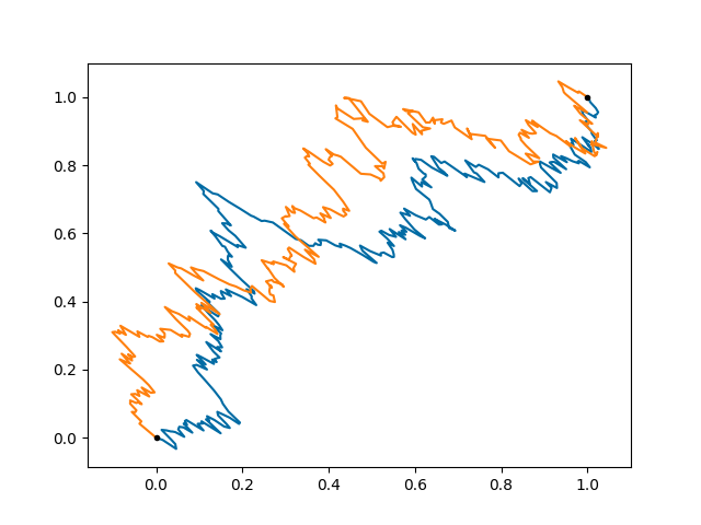
fig, ax = plt.subplots(num='lsqfitgp example')

for sample in gvar.raniter(path, 2):
    ax.plot(sample[0], sample[1])
ax.plot([0, 1], [0, 1], '.k')

fig.savefig('out1.png')

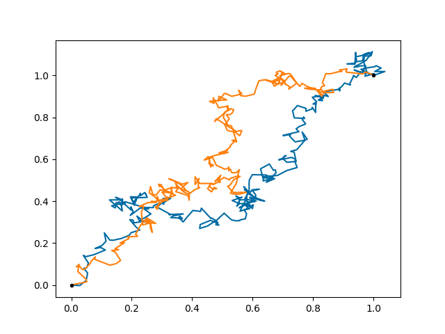
The paths go quite directly to the endpoint. This is because we allowed a total time of only 0.1. Let’s see how far would it go a priori:

prior = gp.prior('walk')

for sample in gvar.raniter(prior, 2):
    ax.plot(sample[0], sample[1], linewidth=1)

fig.savefig('out2.png')

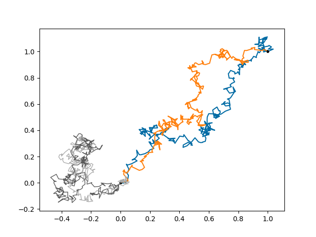
Not so far as (1, 1) indeed. Can we make the task even harder for our walker? We can introduce an anticorrelation between the x and y components, such that going directly in the top-right direction is unfavored.

corr = -0.99
cov = np.array([[1,    corr],
                [corr, 1   ]])
gp = (lgp
    .GP(lgp.Wiener(dim='time') * lgp.Categorical(dim='coord', cov=cov))
    .addx(x, 'walk')
    .addx(end, 'endpoint')
)

path = gp.predfromdata({'endpoint': [1, 1]}, 'walk')

ax.cla()

for sample in gvar.raniter(path, 2):
    ax.plot(sample[0], sample[1])
ax.plot([0, 1], [0, 1], '.k')

fig.savefig('out3.png')